Table of Contents
- The structure database
- How MODELLER works
- Why MODELLER works
- anvi-gen-structure-database
- Description of all MODELLER parameters
- A quick case study on the importance of key parameters
- Using the structure database as an input to anvi-gen-variability-profile
- Display metagenomic sequence variants directly on predicted structures
- Conclusion
The contents of this post assume you are working with anvi’o v7 or later.
This is a theoretical tutorial describing the details of the structure database, how it’s created, and its utility. For a more practical tutorial that demonstrates some of the same concepts, and a thorough walkthrough of the anvi’o structure interactive interface, please visit the Infant Gut Tutorial.
To me, the most fascinating thing about proteins is how specifically they associate with their ligands to carry out their function, and yet how they all kinda look the same. An alpha helix here, a beta sheet there, couple of loops connecting the two, but overall just a big glob of polypeptide chain. The arbitrariness of protein shape is the reason that it’s so surprising to me that these proteins don’t just promiscuously interact with everything around themselves, aggregating to become toxic biohazards inside the cell. Yet of course we know they don’t do that. We know they are finely tuned by natural selection to interact specifically with their ligands and that even a single mutation in the right place can destroy this functionality, leading to a potentially detrimental fitness decrease of the cell and elimination from the population. This is life.
So it’s true that proteins are extremely sensitive to certain mutations. But they are surprisingly robust to others, and it is this permissibility of neutral mutations that leads to the majority of amino acid and codon sequence diversity observed in microbial populations. This tutorial will introduce how you can use environmental metagenomes and short read recruitment strategies to gain insights into the sequence variation within microbial populations, how this variation maps to their protein tertiary structures, and how it is governed by principles of evolutionary biochemistry.
This is all made possible with anvi’o structure, and the meat of the workflow is just two
commands. The first command, anvi-gen-structure-database, predicts protein structures
encoded by genes present in a contigs database and stores the resulting structures in a structure
database. Once this is done, variation from a profile database can be visualized onto the structures
with the command anvi-display-structure. From within the interface one can interactively filter and visualize
variants overlaid on the structure. It’s really that easy.
The itinerary for this post is to first discuss the structure database in-depth, and then explain how to interactively visualize environmental variants on protein structures.
The structure database
This section provides an overview of how protein structures are predicted, the commands responsible for doing so, the user tunable parameters to refine how your structure database is created, and finally the effects they have on structure accuracy.
We, the developers of anvi’o structure, are not structural biologists and we claim no authority on reference-based protein homology modelling. Under the hood, anvi’o structure uses the structure prediction software called MODELLER, a long-standing gold standard in protein prediction. In part, the effort of anvi’o structure is to make this powerful approach accessible to microbial ecologists and their data. But if you disagree with what were saying, please tell us.
How MODELLER works
How does MODELLER work? This paper dissects the MODELLER workflow into four major steps which are summarized here:
-
Alignment. Sequences from a database of proteins with known structure are aligned to your query protein (aka your target protein) sequence, and the database sequences with notably good alignments are stored as candidate templates.
-
Template selection. From this list of candidate templates, some number are selected to be structural templates that your target structure will be modelled from. The selection is done either with automated criteria or ideally through meticulous, manual intervention. Note that several templates can be used to model your target structure.
-
3D-alignment. Your target sequence is aligned in 3D space to the known structures of your templates. You can think of this as “threading” your 1D sequence into a 3D space.
-
Satisfy spatial restraints. The alignment structure from step 3 is the initial configuration for a simulation which perturbs the atomic positions of your protein iteratively to solve an optimization problem. The optimization minimizes the likelihood of a many-dimensional probability density function that compares C alpha-C alpha distances, main-chain N-O distances, main-chain and side-chain dihedral angles in your protein to the distribution of values found in a large database of reference protein structures. The simulation is run until the structure settles into an equilibrium, and the final state is your predicted structure. If you are specifically interested in this step, you should also check out the original MODELLER paper here.
If you think this is amazing, the scientific community agrees with you; MODELLER has been cited more than 10,000 times, and has remained relevant to the community for over 25 years.
Why MODELLER works
MODELLER and similar programs make use of protein homology modelling and reference structures to stitch together a predicted structure. This approach is successful for two main reasons:
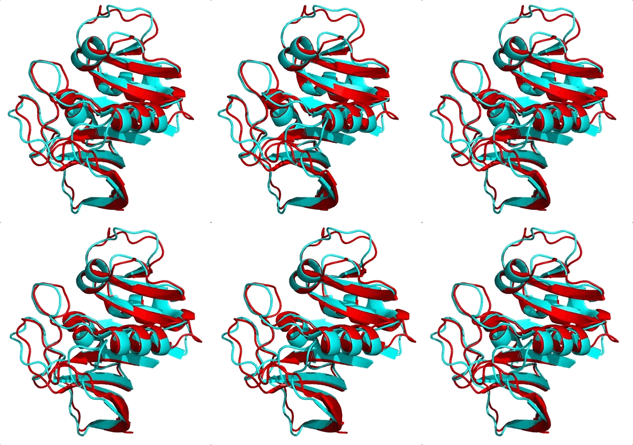
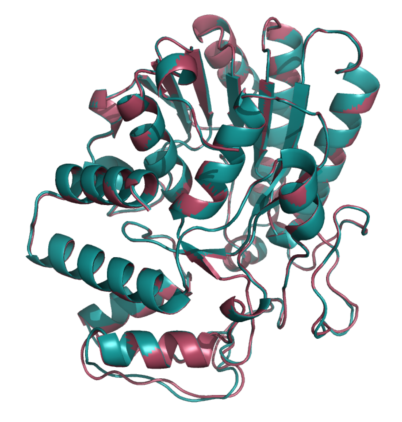
The first is the surprising fact that structure is much more conserved than sequence. Let me ask you a question. Shown below are the structures of two nearly equal-length proteins I have overlaid on top of each other. Based on their obvious structural similarity, what percentage of amino acids would you guess are identical? To say it another way, if you move along the sequence of one protein, what percentage of residues would match with the other protein’s residue at the same position?
I’ll let you think know about it…
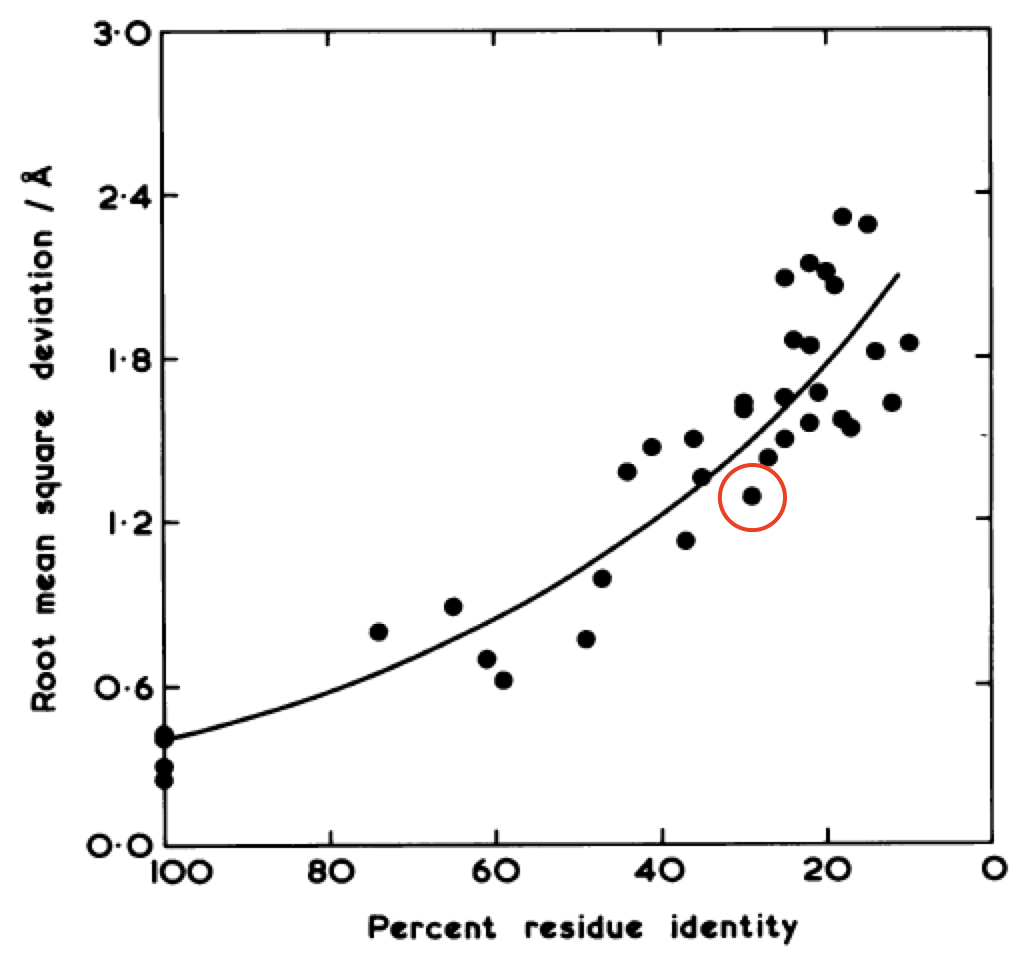
These two proteins are 3DFR and 4DFR and you may be surprised to know that they only share 29% sequence identity, with a root-mean square difference (RMSD) between their main chain atoms of 3.927 Å. Visually, you can see that it is not much difference. In the paper from which I found these proteins, they looked at a total of 34 pairs of homologous proteins (which was totally badass in 1986) and they found the following relationship between sequence similarity and RMSD:
In red I’ve circled the above comparison. The RMSD is lower than the previously reported value of 3.927 Å because they only performed the calculation on a subset of the atoms. The results quite boldy show that RMSD is conserved even over significant sequence divergence. My interpretation of these results is that the “metastructure” for a protein family corresponds to an island in sequence space, and protein sequences in the family evolve happily within the confines of the island, which is more than spacious enough for functional diversification. Yet if any protein sequence drifts off of the island (i.e its structure becomes too dissimilar from the metastructure) it faces detrimental fitness costs brought on by the open ocean (i.e. being unable to fold or remain stable) and is unable to cope. So virtually all sequences remain on the island, because its too difficult to get off, and hey, there’s palm trees so things here aren’t so bad.
Anyways, that’s the first main reason why template-based homology modelling approaches work. The second reason is that there exists a lot of solved structures that can be used as templates to predict the structure of your target sequence. In my brief experience using E. faecalis and SAR11 genomes, approximately half of the genes had sequence matches above 30%. However, please keep in mind the following law of the universe: the more you want a gene to have a homologous structure, the less often it does.
Based on the results of this MODELLER paper, as well as several protein experts I’ve talked to, 30% sequence similarity with few extended gap regions is around the lower limit of when structures can be modelled through homology and the results can be trusted to within a couple ångströms. Obviously, drawing parallels between characteristics such as binding pocket geometry should be taken with a grain of salt at this level of similarity, as functions can differ drastically.
anvi-gen-structure-database
So you want to predict some structures for some genes you’ve identified as interesting, eh? All you need is a list of those gene IDs and the contigs database in which they are described. This is the simplest form of this command:
anvi-gen-structure-database -c path/to/your/CONTIGS.db \
                            --gene-caller-ids 1,2,3 \
                            -o STRUCTURE.db
Where path/to/your/CONTIGS.db is the file path of your contigs database, -o STRUCTURE.db states
that the database will be named STRUCTURE.db, and 1,2,3 are three genes you are interested in,
identified by their gene caller IDs, and separated by commas (no spaces). Alternatively, you could
make a file that is a list of genes caller IDs of interest:
1
2
3
And run the command
anvi-gen-structure-database -c path/to/your/CONTIGS.db \
                            --genes-of-interest path/to/your/genes/of/interest.txt \
                            -o STRUCTURE.db
Finding templates with DIAMOND
When anvi-gen-structure-database is first ran, a DIAMOND database internal to anvi’o will be
created that contains the sequences of all PDB amino acid sequences clustered at 95% similarity to
remove redundancies. This collection of sequences, which the DIAMOND database is created from, is
hosted and maintained by the Sali Lab (the group that develops MODELLER), and which they have called
the pdb_95 dataset.
With this in place, matches to the DIAMOND database will be identified for each gene of interest.
Obtaining template structures
If any templates are found, anvi-gen-structure-database will obtain their structures. How that is done depends on
whether the user has ran the command anvi-setup-pdb-database, which creates a roughly 20GB
database containing the .pdb files of each and every sequence in the DIAMOND database. If they
have ran this command in the past, the structures will automatically be fetched from this database.
Otherwise, the default behavior is to download the structures directly from the RCSB server using an
internet connection. It does not matter in the end how the structures are obtained, as long as they
are obtained, however the advantage of running anvi-setup-pdb-database is avoiding the requirement
of an internet connection.
Whichever the method, anvi-gen-structure-database will invoke MODELLER, and MODELLER will try its best to predict a
structure based on the templates. Everything from the templates used to the quality scores of the
protein models will be stored in the structure database, along with the structures themselves.
Description of all MODELLER parameters
Okay so you know how to make a simple structure database, but MODELLER has many parameters that are waiting to be refined.
We have tried our best to make as many parameters tunable as possible to create the databases you want and with the level of stringency that you control. Below are a list of all the parameters that you can use to fine-tune database creation.
If you use MODELLER and there’s something you want to control but that we don’t provide access to, please let us know and we’ll try our best to add it.
-
--num-models. As already described, once MODELLER has 3D-aligned the target to the templates, it carries out an optimization simulation. This process is deterministic, meaning that if you run the simulation 3 times with the same initial structures, the 3 final structures (aka models) will be the same. Yet if you perturb the atomic positions of the initial structure before running the simulations (see--deviation), you may stumble upon different, and perhaps even better, models. Therefore, it makes sense to simulate several models to search a larger solution space. This parameter controls the number of models to be simulated. Keep in mind that protein templates are the largest determinant of a model’s accuracy, so there is no need to go overboard with large numbers. The default is 1, but feel free to use more. -
--deviation. The standard deviation of atomic perturbation of the initial structure in ångströms. You can explore more of the solution space by perturbing the atomic positions of the initial structure. The default is 4. -
--modeller-database. MODELLER finds candidate template sequences from a sequence database of proteins with known structures. By default, it uses a database,pdb_95, which contains the sequences of all PDB structures clustered at 95% sequence identity, which can be downloaded here. It’s a very convenient resource and is periodically updated by the Sali Lab. If you don’t have it, anvi’o will download it for you when the time is right. If you have your own database it must have either the extension.bin,.piror.dmndand anvi’o should be able to find it underanvio/data/misc/MODELLER/db. -
--scoring-method. If you generated 10 models with--num-models 10, how should the best model be decided? The metric used could be any ofGA341_score(citation),DOPE_score(citation), ormolpdf, which is the simplest scoring function.GA341is an absolute measure, where a good model will have a score near1.0, whereas anything below0.6can be considered bad.DOPE_scoreandmolpdfscores are relative energy measures, where lower scores are better.DOPEhas been generally shown to distinguish better between good and bad models compared tomolpdf. MODELLER usesDOPE_scoreby default. To learn more about assessment methods, see this MODELLER tutorial here. -
--percent-identical-cutoff. Minimum normalized percent identity of a PDB protein to be used as a template for a given gene. Here we define normalized percent identity as the percentage of amino acids in the gene of interest that are identical to an entry in the database given the entire length the protein of interest. For example, if there is 100% identity between the protein of interest and the template over the length of the alignment, but the alignment length is only half of the protein of interest sequence length, then the normalized percent identical would be 50%. This helps us avoid the inflation of identity scores due to partial matches. The default is 30%. Obviously the higher the percentage identity, the more confident you can be in the accuracy of the model, however it will reduce your hits. Keep in mind that if you are after high accuracy, selecting template structures based on a single threshold is very simplistic. The template selection step is perhaps the most critical aspect of the workflow, and requires manual intervention if accuracy is critical. -
--max-number-templates. Generally speaking it is best to use as many templates as possible given that they have high proper percent identity to the protein of interest. Here is an excerpt from the Sali Lab: “The use of several templates generally increases the model accuracy. One strength of MODELLER is that it can combine information from multiple template structures, in two ways. First, multiple template structures may be aligned with different domains of the target, with little overlap between them, in which case the modeling procedure can construct a homology-based model of the whole target sequence. Second, the template structures may be aligned with the same part of the target, in which case the modeling procedure is likely to automatically build the model on the locally best template [43,44]. In general, it is frequently beneficial to include in the modeling process all the templates that differ substantially from each other, if they share approximately the same overall similarity to the target sequence”. The default is 5, but if only X candidate templates are found to pass the--percent-identical-cutoffthreshold, then only X will be used. -
--very-fast. Use this option if you’re impatient and want only the roughest predicted structures. It’s fast because the step size of the simulation is very large and a very low quality requirement is established for reaching equilibrium. Not recommended, but we’re not going to be the ones to deny you of freewill. -
--dump-dir. Modelling structures requires a lot of moving parts, each of which have their own outputs. The output of this program is a structure database containing the pertinent results of this computation, however a lot of stuff doesn’t make the cut. By providing a directory for this parameter you will get, in addition to the structure database, a directory containing the raw output for everything produced by MODELLER.
A quick case study on the importance of key parameters
How much do these parameters matter? In this section we look at a gene from a SAR11 genome that encodes for CDP-D-glucose 4,6-dehydratase, and investigate the effect of template selection and model number on the predicted structure.
How much does the number of models matter?
This is anecdotal, and represents only 1 case.
Hopefully it’s clear that increasing the number of models increases the search space and the
accuracy of your final model, but when is enough, enough? To test this I predicted the SAR11
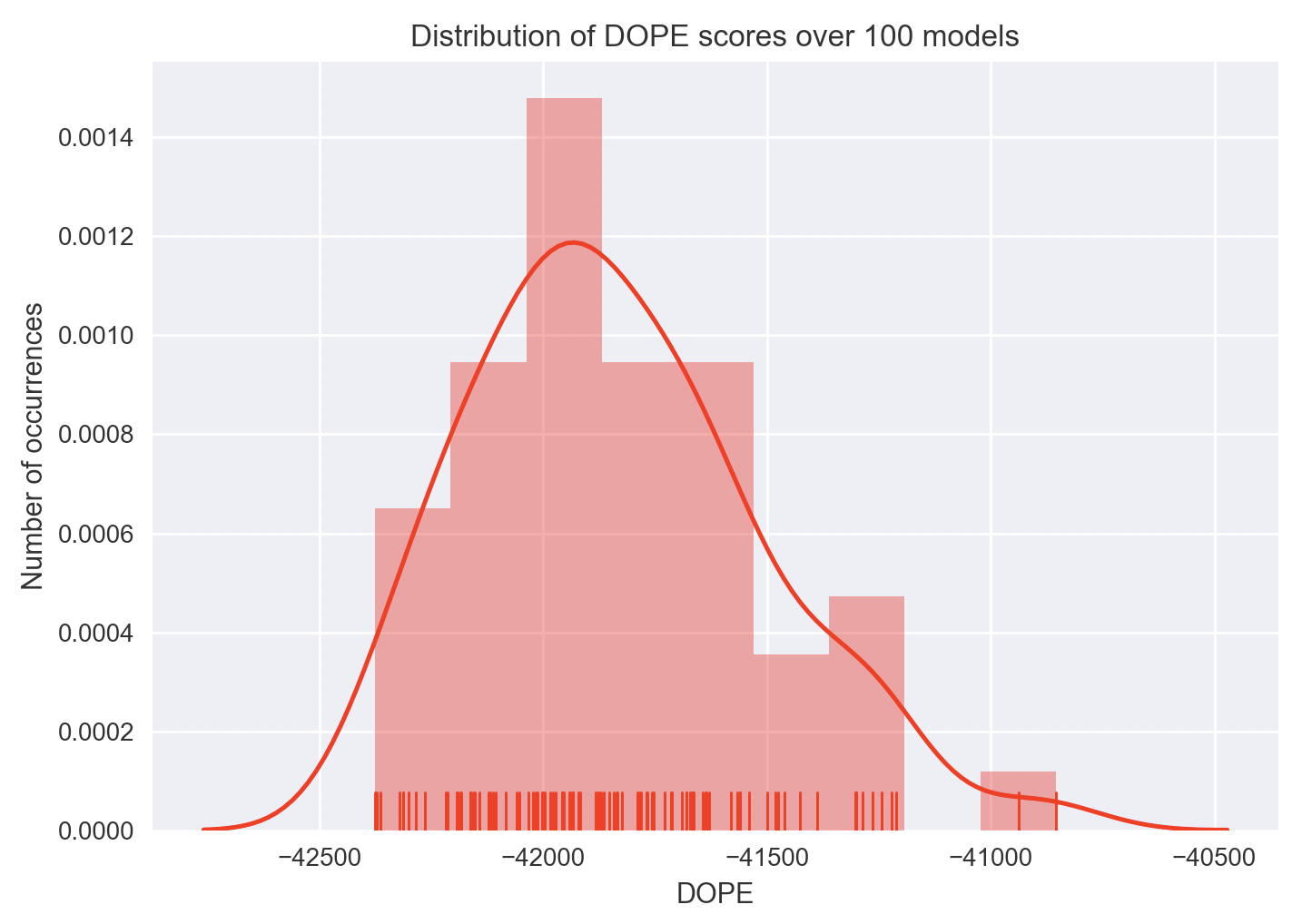
dehydratase structure with default parameters except with --num-models 100. Here are the DOPE
scores of those 100 structure predictions, which took about an hour to compute:
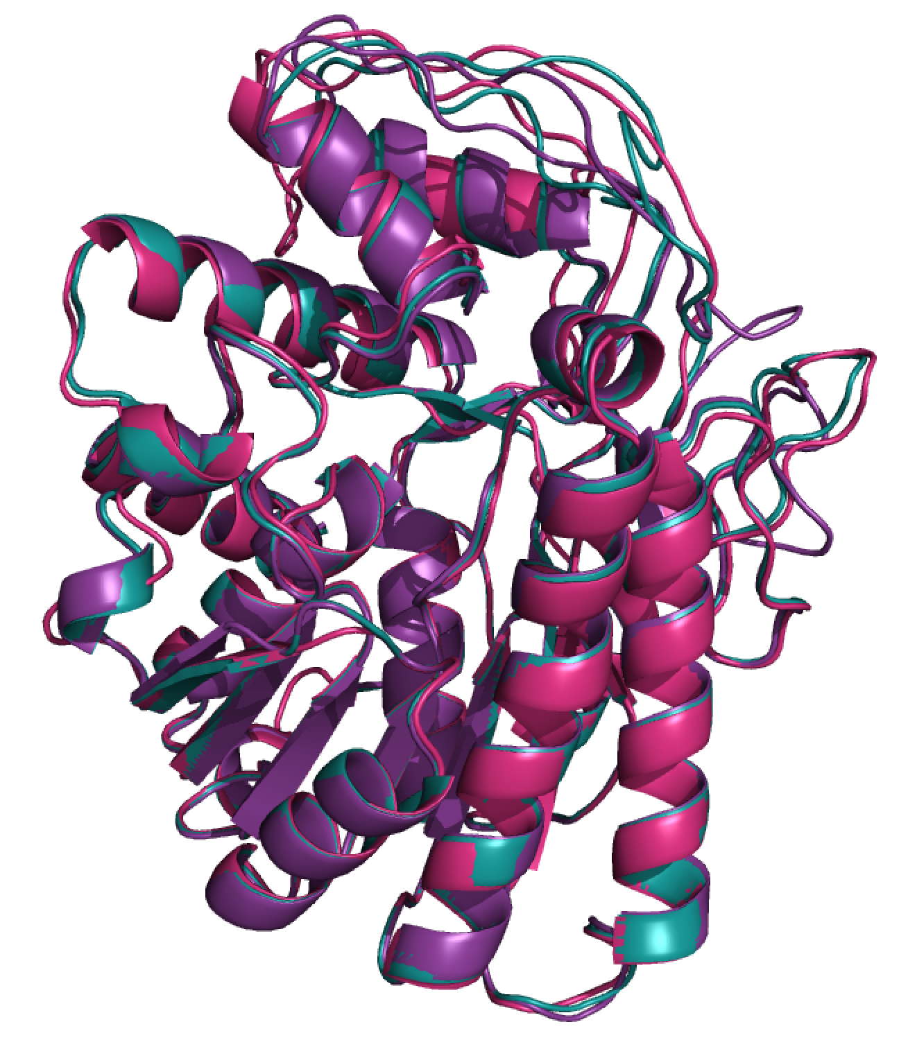
Since model 79 has the best DOPE score of -42376.1132812 (most negative), it was picked as the best model. But that’s just a number, and I certainly don’t know how to meaningfully compare models using this score besides comparing their magnitudes. So here is a visual comparison between the best and worst models according to DOPE score:
They have an RMSD of 1.617 Å. I will let you be the judge of how different these are, but in general
keep in mind it will depend on what questions you are interested in. Based on the visual similarity
between the two models in this case study, the default value for --num-models has been set to 3.
How much do templates matter?
This is anecdotal, and represents only 1 case.
The higher the similarity of your templates to your target, the better your model will be. But how does the effect of multiple templates influence model results? Let’s see.
For this SAR11 dehydratase gene, MODELLER finds 2 candidate templates above 30% identity:
Template 1 ........................: Protein ID: 1wvg, Chain A (39.4% identical)
Template 2 ........................: Protein ID: 1rkx, Chain A (38.8% identical)
Template 1 comes from Salmonella typhi and template 2 from Yersinia pseudotuberculosis. They are
both ~39% similar to SAR11 but 73% similar to one another, with a RMSD of 2.053 Å between their
main-chain atoms. I created 3 different models, one using template 1, a second using template 2, and
a third using templates 1 and 2. Figure below shows the best models (using --num-models 15) from
each of these 3 templates.
Visually it’s clear that there are differences between these models that could be considered either very significant, or very insignificant –it depends what you’re interested in. If you want to classify which residues are in the hydrophobic core versus on the surface of the protein, these are all essentially equivalent models. If on the other hand, you are trying to define the precise geometry of a binding pocket, these differences will be critical to understand.
Here is a table quantifying RMSD between each pair (in ångströms):
| Templates used | 1rkx | 1wvg | both |
|---|---|---|---|
| 1rkx | - | 4.429 | 4.304 |
| 1wvg | - | - | 2.617 |
| both | - | - | - |
So which model is best? Looking at the DOPE scores,
| Templates used | DOPE |
|---|---|
| 1rkx | -42248 |
| 1wvg | -42209 |
| both | -42362 |
We see that the model based on both templates outperforms both single-template models. This reflects a general rule of thumb proposed by the Sali Lab:
The use of several templates generally increases the model accuracy. One strength of MODELLER is that it can combine information from multiple template structures … the template structures may be aligned with the same part of the target, in which case the modeling procedure is likely to automatically build the model on the locally best template. In general, it is frequently beneficial to include in the modeling process all the templates that differ substantially from each other, if they share approximately the same overall similarity to the target sequence.
In our case, both the Salmonella and the Pseudotuberculosis proteins shared the same overall
similarity to the SAR11 sequence, so utilizing both templates led to a better model. What if there
was a third template that shared 90% similarity to our protein? Should we use all three templates or
should we just use the one with 90% similarity? In this instance, we should use only the one
template with 90% similarity, since the other 2 templates do not share the same overall similarity
to the target sequence, and would lower the quality of our odel. On the other hand, if the third
model was 45-50% similar to the target sequence, using all three could make more sense.
Unfortunately this sort of decison-making is not coded into anvi-gen-structure-databse, and at this point in time
only provides a hard cutoff with --num-templates. Complain to us if this matters to you!
Using the structure database as an input to anvi-gen-variability-profile
Once you have structures for proteins of interest, what can you do with them? One utility is to
combine the output of anvi-gen-variability-profile with structural information.
anvi-gen-variability-profile is a robust program to generate variability profiles for metagenomes
at the level of nucleotides (SNVs), codons (SCVs), or amino acids (SAAVs). You can get a hands-on
feel for this program in this section of the Infant Gut
Tutorial or you
can get into the nitty-gritty in this more theoretical
tutorial dedicated to the subject.
The output of anvi-gen-variability-profile is a table where each row corresponds to a sequence
variant found in a metagenome. Each column gives descriptive or quantitative information about the
variants. If the parameter -s /PATH/TO/STRUCTURE-DATABASE.db is given to the program, additional
columns will be added for structural information if (a) the variant occurs within a gene, (b) the
gene has a predicted structure, and (c) the variant is either a SAAV (use --engine AA) or an SCV
(use --engine CDN). All the columns that can be added are listed
here.
This is my favourite feature of the structure database.
Display metagenomic sequence variants directly on predicted structures
anvi-display-structure, described below, visualizes variability from metagenomic sequence data onto a reference
3D structures. The structures are predicted either from a MAG or a reference genome with
anvi-gen-structure-database. This program does not predict the impact of environmental variants on
the structure.
There are many comprehensive software packages and web services to visualize protein structures. But Özcan and I wanted to create anvi’o structure with the very specific purpose of interactively visualizing, filtering, and clustering metagenomic sequence variants directly on protein strucures. Existing solutions were not incapable of doing these tasks, however, the lack of automation, scalability, and just the straight up time required for a single protein and the lack of integration convinced us that the community could benefit from a tool that was designed specifically for this purpose.
Examples
Details describing the interface itself are provided in a hands-on demonstration within the infant gut tutorial, which I highly recommend you to follow either with the tutorial data or your own. But the tutorial you’re currently reading wouldn’t be complete if we didn’t at least showcase some images and movies from the interface. With this in mind, check out this video demonstration below of some of the features of the interface.
As well, feel free to view the screenshots below with their accompanying descriptions.
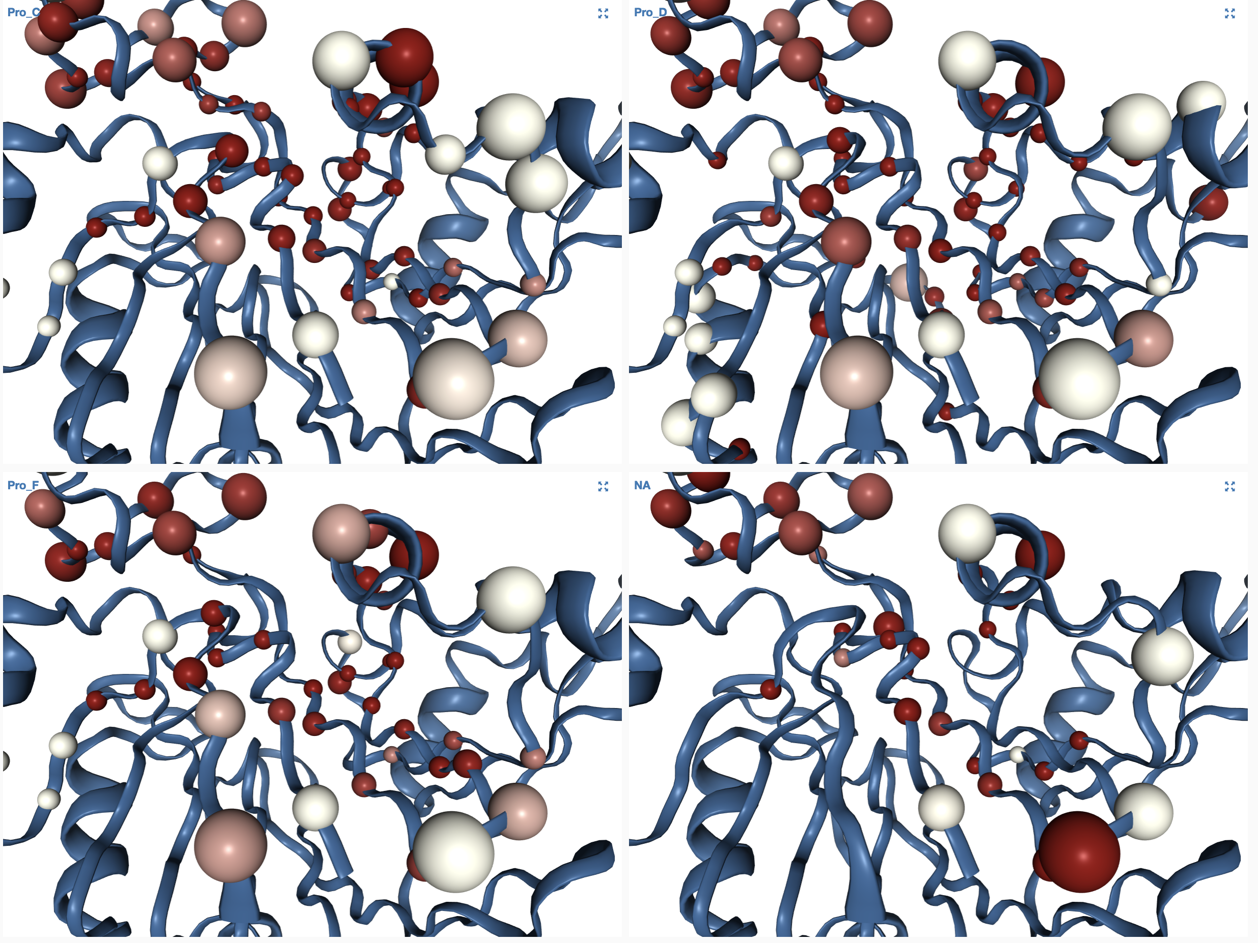
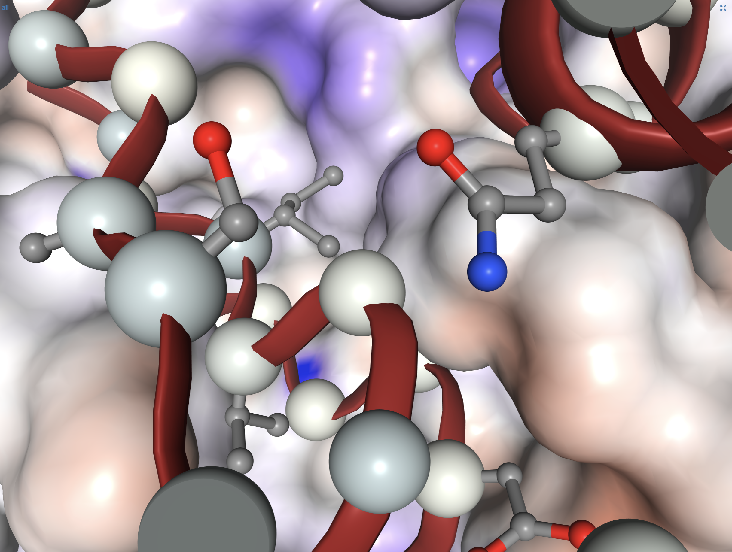
Above is a protein from a reference SAR11 genome called HIMB83. Each of the 4 views correspond to groups of TARA ocean metagenomes organized by the user. Each sphere on the structure corresponds to a SCV that occurred in at least one of the metagenomes of the group. The size of each sphere relates to the solvent accessibility of the residue (aka how exposed to water it is) and the color of each sphere corresponds to the SCV’s synonymity. The trend demonstrates that solvent inaccessible residues are under high purifying selection against non-synonymous mutations, but readily permit synonymous mutations as they do not compromise protein stability.
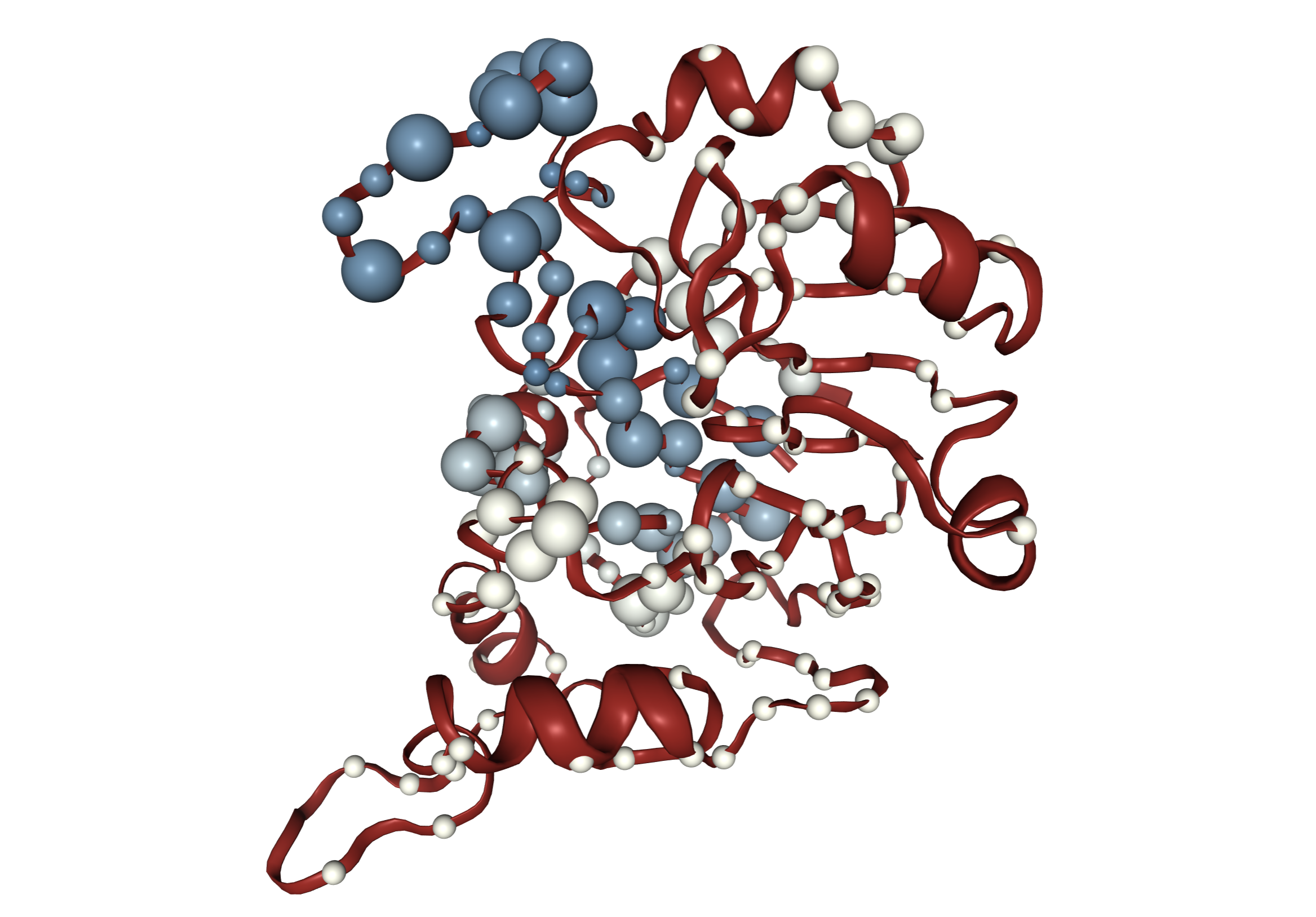
Above is a merged view of all TARA ocean metagenomes for the same protein. The size of each sphere refers to the fraction of metagenomes in which the position was a SCV (e.g. the smallest spheres occur in only one metagenome). We see that one region of this protein is significantly more variable than the other. The color refers to the coverage of that site normalized by the average gene coverage for a metagenome. This indicates that the hypervariable region is also recruiting much more reads than the others, as a result of non-specific mapping.
These protein views are interactive with many visualization options. For example, above we have zoomed in to a specific region and visualized the side chains of SCVs that are in close proximity to one another.
Supplying anvi-display-structure with sequence variability
Please note that the only required input for creating a structure database with
anvi-gen-structure-database is a contigs database. But to visualize sequence variants on
structures in your structure database, you will also need a single or merged anvi’o profile database
that must have been generated with the flag --profile-SCVs, as this flag is what makes reporting
SCVs and SAAVs possible. Otherwise, anvi’o will complain, and complaining has never solved any
problem. If you have profile databases without this flag and want to visualize variants on
structures, you have to re-profile with --profile-SCVs. We apologize for the inconvenience, but
the reason this is not done by default is that it comes at a large computational cost.
The remainder of this tutorial describes the two ways in which you can provide anvi-display-structure with
sequence variability information, which is required to run the interface. The easiest and most
straightforward way is to not provide anything, and let anvi’o do it for you. Simply provide
the corresponding contigs and profile databases alongside your structure database:
anvi-display-structure -s /PATH/TO/STRUCTURE.DB \
                       -p /PATH/TO/PROFILE.DB \
                       -c /PATH/TO/CONTIGS.DB
In this case anvi-display-structure will calculate both SCVs and SAAVs on-the-fly and the following messages will appear in your terminal:
* SAAVs for gene X are loaded
* SCVs for gene X are loaded
Afterwards, the interface will open a display for gene X. Notice that SCVs and SAAVs were only calculated for gene X. If you switch genes in the interface, SCVs and SAAVs will be calculated for the new gene.
This is the standard way to visualize variation and is recommended in most cases. But there is an
additional way that could be useful for one of two reasons: (1) profiling variation on-the-fly can
take a long time for large profile database (on my laptop it takes about a minute to load each gene
in a 26 GB profile database), and (2) if you merely want to show someone variation in a gene across
some metagenomes, you don’t want to send them a 26 GB profile database. Why not just send them a
variation table? Hence, the second way to provide anvi-display-structure with sequence variability is with a
variability table generated from anvi-gen-variability-profile. With this approach, anvi’o will
utilize variability from this table instead of reading it from the profile database:
# generate a variability table
anvi-gen-variability-profile -p /PATH/TO/PROFILE.DB \
                             -c /PATH/TO/CONTIGS.DB \
                             -s /PATH/TO/STRUCTURE.DB \
                             --engine AA \
                             --only-if-structure \
                             -o variability.txt

# run the display using the variability table
anvi-display-structure -s /PATH/TO/STRUCTURE.DB \
                       -V variability.txt
The first command has some bells and whistles that are worth describing. First, -s
/PATH/TO/STRUCTURE.DB is provided so that the structural information is added into the variability
outuput. Second, the flag --engine AA tells anvi’o to report SAAVs (for SCVs or SNVs you cold use
CDN or NT, respectively). Thirdly, --only-if-structure subsets your genes of interest to only
include those with a structure in the structure database. That means if you have 1000 genes in your
contigs database but only 3 have structure, variability will only be generated for those 3. Finally,
-o variability.txt is the name of the output file.
Once variability.txt is generated, the second command feeds it into anvi-display-structure along with your structure database. A warning will pop up that is reiterated here:
WARNING
===============================================
You opted to work with a variability table previously generated from anvi-gen-
variability-profile. As a word of caution, keep in mind that any filters applied
when the table was generated now persist in the following visualizations.
Conclusion
We hope that this tutorial has been useful for you. If you have any suggestions or questions please post an issue on GitHub or join our Slack channel.
