


Table of Contents
This workflow is for v6 and later versions of anvi’o. You can identify which version you have on your computer by typing anvi-self-test --version in your terminal.
“Read recruitment”, “read mapping” or even just “mapping” are thrown around all the time in metagenomic studies and they all describe the same thing. If you already feel confident with read recruitment, feel free to skip down to the new stuff, probably starting at the section “Visualizing coverage data in anvi’o”.
But if you want a refresher, here we start with a quick summary about the underlying principles and the utility of one of the most powerful strategies that we frequently rely on in metagenomic studies to make sense of environmental populations.
How does read recruitment work?
Understanding superficially how read mapping works is fairly straightforward. You have one or more genomes, or contigs assembled from metagenomes as your reference, and you’re figuring out how many of your short reads in your metagenomes match to your reference sequences. Like the animation below shows, you can do this for multiple metagenomes (i.e., multiple samples) and study the distribution of a given reference sequence across environments. It also gives you important information like the coverage or the detection of your reference.
Intuitively, you can think of mapping as the process of taking a metagenomic read, determining whether it matches any of the reference sequences, and placing it neatly under the part of reference to which it matches best, and doing this for every single read. That’s exactly what coverage plots display: how short reads align to a reference context. Often, this level of understanding is good enough for a lot of things. But this is not exactly how things actually work. While this exact description of mapping would work in theory, in practice finding the best matches of each short read through alignment is incredibly computationally intensive. Instead, all popular software used for read recruitment use some fancy approaches to dramatically increase the speed of mapping.
If you’re interested, the remaining text in this section will provide a short summary (to the best of our understanding) of how a mapping index is made, and how the reads are aligned.
For this summary we have extensively relied upon this video and the original Bowtie paper. The slides that accompany the video can be found here. This is a biologist’s understanding and introduction to the complexities of mapping, and by no means a full explanation. If you’re interested in learning more in depth how this process works, see one of the original references listed in this paragraph.
In our lab we frequently use Bowtie2 to recruit reads, so this explanation will be in the context of Bowtie2. That said, most read mapping software use similar techniques.
Typically, you start with a reference file input in FASTA format. For simplicity, let’s say our FASTA contains a single reference genome. Bowtie2 takes this FASTA file and uses a Burrows-Wheeler Transformation to convert it to a Bowtie2 index. This is a method of compressing your data by cyclically rotating the sequence to get all possible rotations of the sequence, ordering them alphabetically, ranking each letter by its occurrence, and keeping only the right most column of data. The ordering means that the rank, the nth time that that letter has appeared in the sequence, is the same in the first and last columns. The letters are also assigned a count value, in other words their original position in the sequence. We can use the Last to First (LF) function to match a character with its rank (these values are stored by the algorithm) and use the Walk Left function to reconstruct the initial sequence from these data. More information on these functions can be found here.
Ok, so now we have a Bowtie2 index, how do we actually map the reads? Our input reads will typically be in FASTQ format, so we’ll have the read information and a quality score for each base. To find reads that match exactly, we use something called a Full-text index in Minute space (FM) index. This matches your read from right to left (5’ to 3’) to the Bowtie2 index. Each iteration of top and bottom using the FM index indicates the range of rows in the index that have progressively longer matches to our query read. If the range is 0, it means that there’s nothing that matches the read sequence exactly and it wouldn’t be mapped. But we can immediately think of a problem here. What if there are sequencing errors in our data, or more importantly, true biological variation? We want to be able to map reads that aren’t a perfect match. To get around this, Bowtie2 uses a backtracking alignment search. When it encounters a mismatch, it attempts to add all of the different bases to see what matches and then continues. It can also try to backtrack to the lowest quality match, replace this with another base and continue from there. The number of mismatches and amount of backtracking is limited to avoid reads mapping that do not belong in that position. This algorithm is “greedy”, meaning it will keep the first mismatch that works but not necessarily the best one. Bowtie2 can be forced to use the best one by supplying the flag --best. Because Bowtie2 restricts the amount of backtracking, it may seem like it is biased toward the right hand side of the read, however the left hand side of the read is typically higher quality, and Bowtie2 can use a mirror index to avoid this bias. A mirror index is the reference sequence reverse complemented and made into a Bowtie2 index, then mapping reversed reads to this index. Again, see here for more information.
Alright, the reads have now been mapped, but where are these reads in the reference? To determine this, we take the suffix array, or in other words the file that was generated that kept track of the position of every base in the original sequence. Unfortunately, this complete file is very large, so instead of keeping the entire thing, Bowtie2 keeps every 32nd entry (this number can be adjusted) and then uses the Walk-Left function (which reconstructs the initial sequence) until it hits the suffix of interest.
Yay! The reads are mapped. Now on to the biologically relevant part of the post.
Why are we looking at coverage plots?
We often use read recruitment results to make estimates of relative bacterial abundance. We can tell what percentage of the reads in a given metagenome was aligned to a given section of the reference DNA. In anvi’o, we can show exactly where the reads mapped and how many mapped to each nucleotide position by visualizing coverage plots from the inspect page:
This particular figure shows the coverage of a contig assembled from a human gut metagenome. By just looking at this image you can see that looking at the coverage patterns in a given context is often more insightful than just working with the the mean coverage of that reference sequence. Through the coverage patterns we can tell if the entire reference is covered evenly, or if all the reads are being recruited to one section, thus inflating the mean coverage. Although, if most reads are mapping to one section of the contig this can be biologically interesting too! The mean coverage of this contig is probably around 25X, but even a quick glance at this tells us that the number 25 is pretty meaningless. The depth of coverage of the first section of this contig is ~100X, but the rest of the contig looks like it has ~10X coverage at best. If we take a mean coverage value of 25 it suggests that all the genes in this contig are present uniformly, which is clearly not the case.
In addition to coverage, we can also use these results to visualize the genomic heterogeneity within a sample by looking at single-nucleotide variants (SNVs). A single-nucleotide variant occurs when a nucleotide in the mapped read is different than the reference (these are the mismatches that were discussed in the section about how Bowtie2 works). In the image above, the SNVs are the green, red and black bars extending up from the x-axis. Green indicates nucleotide difference in the third position of the codon, red indicates a nucleotide difference in the first or second position in the codon, and black is a SNV in a non-coding region. The height of the bar indicates the proportion of reads that have a different nucleotide than the reference. Anvi’o has a powerful infrastructure to study microbial population genetics and to make quantitative statements about monoclonality of a sample, or to identify nucleotides positions that are under selective pressures. But visualizing SNVs and simply looking at them in the context of coverage information is essential for anyone who wishes to wrap their minds around their data before gross quantitative summaries.
If you want to know more about the use of read mapping in genome resolved metagenomics, check out the relevant section of the infant gut tutorial. You can learn more about ecological and stochastic factors that contribute to variation in coverage from this blog post.
Visualizing coverage data in anvi’o
The purpose of this post is not to convince you that manual inspection of your contigs is well worth your time (although we hope you recognize the importance of doing it), but rather to explain new features in the sixth version of anvi’o that make this process manageable - especially if you have a ton of samples.
This post assumes that you have the anvi’o databases for a study of yours in which you have mapped one or more metagenomes to one or more contigs (if you are not familiar with anvi’o please refer to other sources, such as this one to learn about how to get your project into anvi’o). It will walk you through the process of inspecting your splits using anvi-inspect for a quick inspection and anvi-script-visualize-split-coverages to export a PDF of these results.
A quick note: by default anvi’o soft-splits contigs longer than 20,000 basepairs into multiple pieces for to have a balanced view of short and long contigs. In the anvi’o lingo each of these pieces are called “splits”, which you can interact with through various interactive interfaces of the platform. If you have a contig that is shorter than the average split size, the split will be equivalent to the contig.
To make things more interesting, we’ll do a re-analysis of a plasmid described in a recent study by Petersen et al (you will get to download the files if you would like to reproduce anvi’o commands and analyses on your computer).
We chose this dataset due to the simplicity and relevance. In their study, Petersen et al identify a highly conserved and globally distributed plasmid called pLA6 12. The authors suggest that the backbone of the plasmid is conserved, but there is a hyper-variable section that can have variable genes, such as chromate resistance, that appear to benefit bacteria that carry it. The authors also mention that the backbone of this plasmid is conserved across sampling locations, but they do not elaborate in the study how they came to this conclusion, nor do they give the details of their approaches in the methods section of the study. In this post we will use this plasmid as a reference, and recruit short reads from marine metagenomes to substantiate the claims made in this study while learning how to use anvi’o tools to study coverage patterns. For this, we downloaded some of the metagenomes listed in the study, mapped short reads from these metagenomes to the plasmid pLA6 12, and profiled the mapping results using anvi’o.
If you would like to follow the rest of the post on your computer, you can run the following commands on your terminal to download the data and and unpack it:
# download
wget http://merenlab.org/files/ANVIO-DBs-FOR-pLA6-MAPPING.tar.gz

# unpack
tar -zxvf ANVIO-DBs-FOR-pLA6-MAPPING.tar.gz && cd ANVIO-DBs-FOR-pLA6-MAPPING
Conventional way to visualizing coverages
Before jumping into the new programs in anvi’o, anvi-inspect and anvi-script-visualize-split-coverages, let’s go through the tried and true approach of visualizing coverage plots once you’ve opened the anvi’o interface. This introduction will give you a better idea of the utility of anvi-inspect and anvi-script-visualize-split-coverages. If you’re comfortable with inspecting contigs from the interface, feel free to skip this section.
If you run this command,
anvi-interactive -p PROFILE.db \
                 -c CONTIGS.db
Your browser will pop-up with a display similar to this:
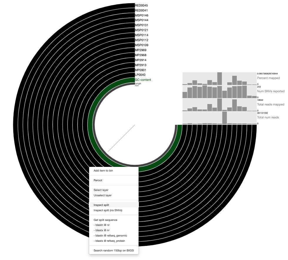
It’s certainly not the prettiest anvi’o figure you’ve ever seen, but we just care about the inspect page here, so let’s move on.
In this display we only have one contig pLA6 12, so we can right-click anywhere and click inspect to open the inspect page which should look like this:
If you had more than one contig, you’d just pick the contig you want to inspect and do the same thing.
Over time we came to the realization that when we have too many samples and contigs to visualize, accessing the inspection page for a given contig in a large dataset can be a significant challenge. That is why, we developed anvi-inspect, which is included in anvi’o since the v6 version.
Targeted visualization of coverage through anvi-inspect
The anvi’o program anvi-inspect enables you to visualize the coverage of a given contig without having to go through the main display of the interactive interface. For this you will need to specify the split name that you’re interested in. There are many ways to find a split name of interest in anvi’o. Programs like such as anvi-search-functions or anvi-export-splits-and-coverages will report split names. But in this particular case there is a single split in our profile database. So we don’t really provide a split name. However, if we run anvi-inspect without any split name, it will not be happy with us:
anvi-inspect -p PROFILE.db \
             -c CONTIGS.db


Config Error: Either you forgot to provide a split name to `anvi-inspect` or the split name
              you have provided does not exist. If you don't care and want to start the
              interactive inteface with a random split from the profile database, please use
              the flag `--just-do-it`
So be it! We shall use the --just-do-it flag and start the interface since the we have a single split:
anvi-inspect -p PROFILE.db \
             -c CONTIGS.db \
             --just-do-it
This command will give you the same inspect page that we saw before, but allows you to skip going through the interactive interface.
So anvi-inspect offers direct access to inspection page and solves some of the problems associated with having to go through the main display when we know which splits we are interested in working with. But over time we reached to another realization: while inspect page is great for interactive visualization with access to all the genes and functions, exporting these coverage plots for publications or presentations is very difficult. One could take screen shots of the inspect page, but that’s not a very elegant solution, nor is it reproducible. And it’s even less ideal if you have a lot of samples.
The next program solves that issue.
Exporting coverage data as a PDF
The new and talented anvi’o program anvi-script-visualize-split-coverages will generate static versions of the coverage plots you see in anvi’o interactive interfaces as a PDF. In other words, this program will give you the inspect page produced in ggplot2. You’ll need the ggplot2 and optparse packages installed in R.
Meren’s note: anvi-script-visualize-split-coverages is the first anvi’o program that is contributed entirely from someone who is not an official member of the UChicago anvi’o headquarters. Ryan Moore, a graduate student at the University of Delaware, heard our call on Twitter, and implemented this lovely program for the entire community. I know I speak on behalf of all anvi’o users who will use his program when I say I am very grateful for his generosity and time. This is how open-source projects grow and become the property of the community rather than being associated with a single group forever. Thank you, Ryan!
The following subsections will demonstrate various uses of anvi-script-visualize-split-coverages and explain how to generate input files for this program using other anvi’o programs.
Visualize only the coverage of a split across samples:
The most basic funcitonality of anvi-script-visualize-split-coverages is to export coverage plots as a PDF. In order to do this, it needs to know the coverage of your split. To get this, you can run the command anvi-get-split-coverages and specify the split name similar to what’s shown below.
If you don’t know what your split of interest is called, you can run this first:
anvi-get-split-coverages -p PROFILE.db \
                         -c CONTIGS.db \
                         --list-splits
Next, you will need to ask anvi’o to export split coverage data so it can be visualized:
anvi-get-split-coverages -p PROFILE.db -c CONTIGS.db \
                         --split-name pLA6_12_000000000001_split_00001 \
                         -o pLA6_12_000000000001_split_00001_coverage.txt
Now it is time to give the output file pLA6_12_000000000001_split_00001_coverage.txt as an input for anvi-script-visualize-split-coverages:
anvi-script-visualize-split-coverages -i pLA6_12_000000000001_split_00001_coverage.txt \
                                      -o pLA6_12_000000000001_split_00001_inspect.pdf
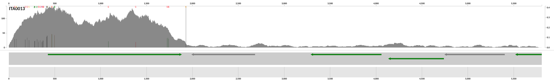
And done! This is a screenshot of the output PDF file generated by this command:
Visualize both coverage and single-nuleotide variants
If you provide the appropriate input file, anvi-script-visualize-split-coverages can plot the coverage values with the corresponding SNVs. The anvi’o program that reports such data from profile databases is anvi-gen-variability-profile. SNVs are essential to have if you want to make statements about sub-populations dynamics of a given environmental poplation or lack there of. This post details the contents of the output file anvi-gen-variability-profile generates. We can ask anvi’o to report the SNV data associated with a given split by running the following command:
anvi-gen-variability-profile -p PROFILE.db \
                             -c CONTIGS.db \
                             --splits-of-interest split_of_interest.txt \
                             --include-split-names \
                             --include-contig-names \
                             -o pLA6_12_000000000001_split_00001_SNVs.txt
Make sure you include the --include-contig-names and --include-split-names flags. The split_of_interest.txt is a plain text file that lists the split names you’re interested in. In our case, the contents of it looked like this:
pLA6_12_000000000001_split_00001
Now we have anvi’o output files both for coverage and SNV data, and are ready to run this command:
anvi-script-visualize-split-coverages -i pLA6_12_000000000001_split_00001_coverage.txt \
                                      -o pLA6_12_000000000001_split_00001_inspect.pdf \
                                      --snv-data pLA6_12_000000000001_split_00001_SNVs.txt
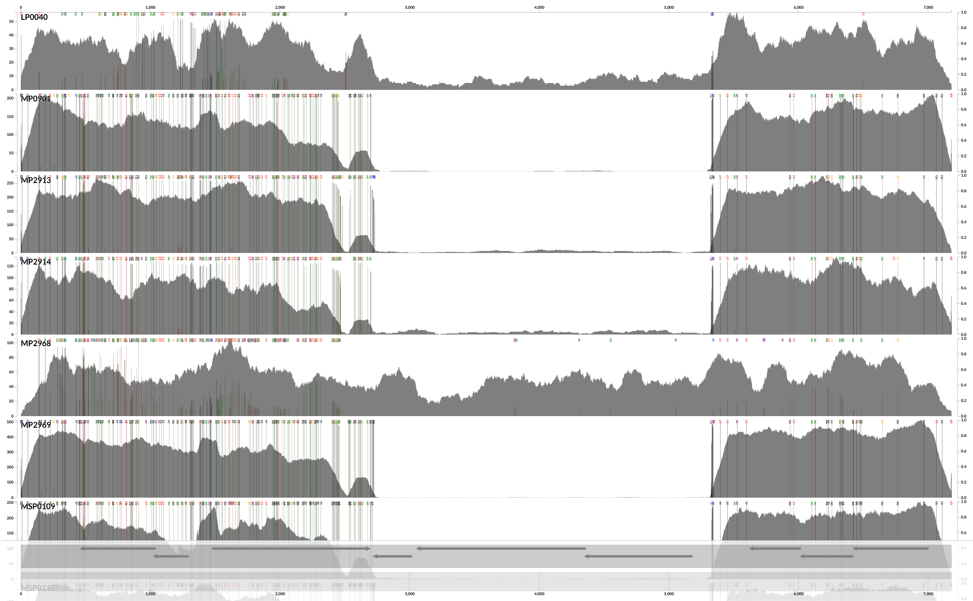
Which creates a PDF file that looks like this:
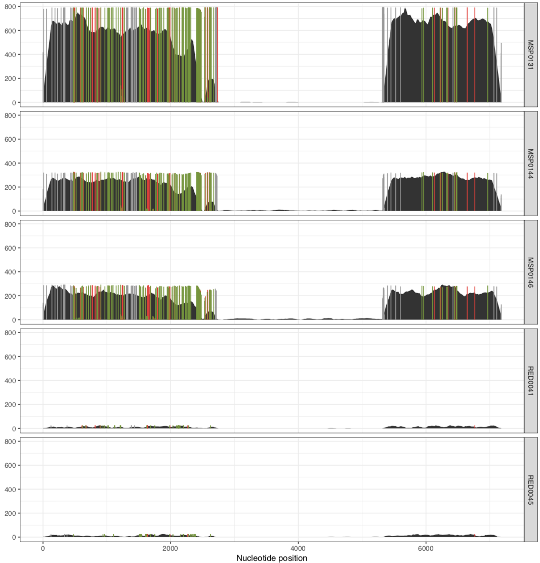
Yay! Now we have SNVs. The default SNV colors are green, red and grey. Green color indicates those nucleotide positions that occur in the third position of a codon. In contrast, red indicates those that are in the first or the second nucleotide position in a codon. As you can imagine, the grey ones are those nucleotide positions that occur at intergenic regions of the chromosome.
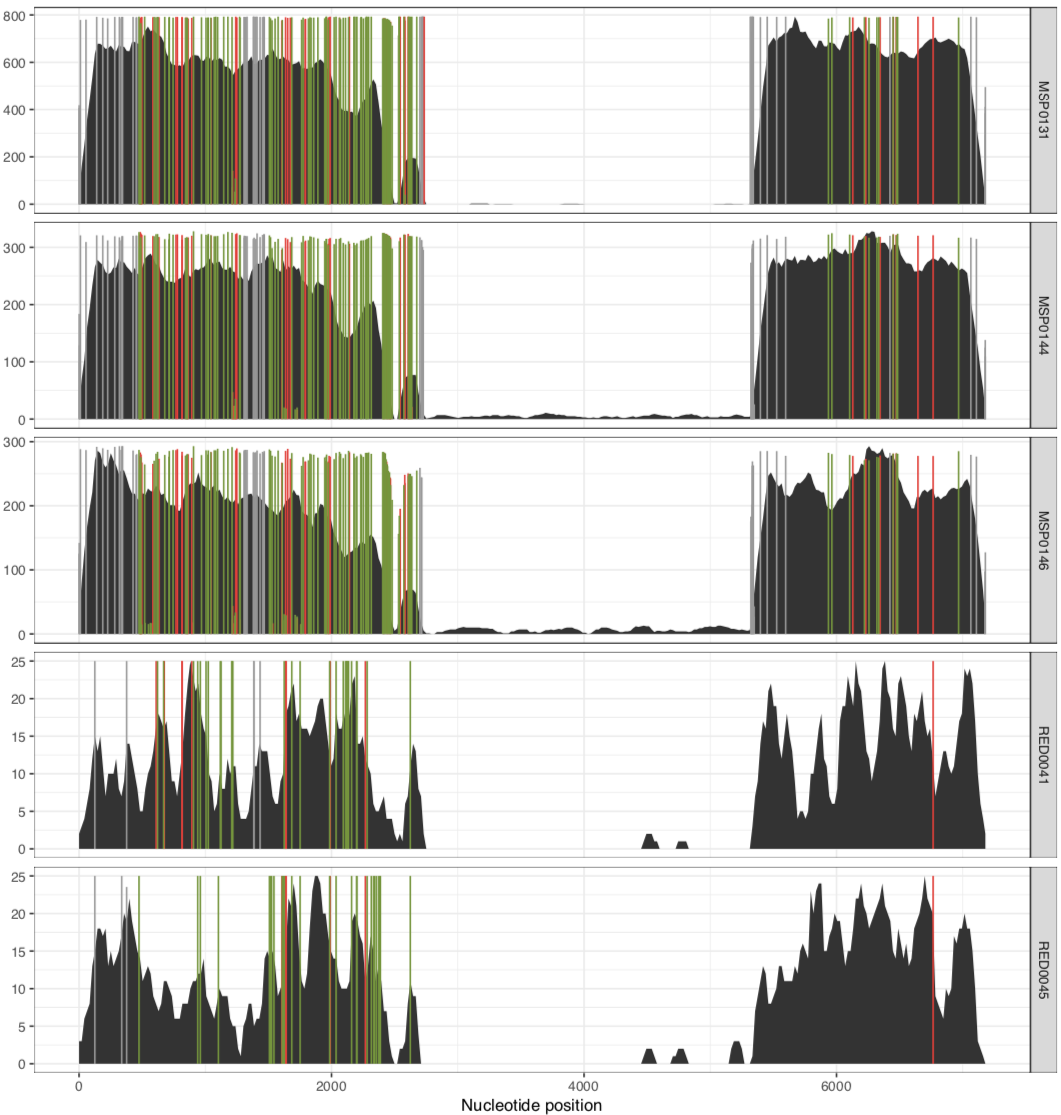
As we can see from the plot above, the coverage in the above samples varies widely, and while this is good to distinguish highly covered vs lowly covered samples, it also makes it difficult to visualize the ones with less coverage, especially if you want to look at SNVs. Thankfully, there is a solution for this. You can run exactly the same anvi-script-visualize-split-coverages command, but add in the flag --free-y-scale.
anvi-script-visualize-split-coverages -i pLA6_12_000000000001_split_00001_coverage.txt \
                                      -o pLA6_12_000000000001_split_00001_inspect.pdf \
                                      --snv-data pLA6_12_000000000001_split_00001_SNVs.txt \
                                      --free-y-scale TRUE
This will give you a plot that looks like this:
Visualize a subset of your samples
Sometimes you may be interested in only a subset of the samples in your profile database. An additional, TAB-delilimited file called samples_data.txt with sample names and their corresponding groups gives you more control on the output PDF, including providing a way to subset your samples.
samples.txt will specify which samples should be grouped together into the same PDF. For example, some of the metagenomes we downloaded were from the Red Sea, and some were metagenomes from pelagic zones all over the world (the Malaspina metagenomes). One could create a file that looks like this to store Red Sea mapping results to one PDF, and the Malaspina metagenomes mapping to another PDF,
sample_name	sample_group
MSP0109	MAL
MSP0112	MAL
MSP0114	MAL
MSP0121	MAL
MSP0131	MAL
MSP0144	MAL
MSP0146	MAL
RED0041	RED
RED0045	RED
and then run anvi-script-visualize-split-coverages this way:
anvi-script-visualize-split-coverages -i pLA6_12_000000000001_split_00001_coverage.txt \
                                      -o pLA6_12_000000000001_split_00001_inspect.pdf \
                                      --snv-data pLA6_12_000000000001_split_00001_SNVs.txt \
                                      --sample-data sample_data.txt
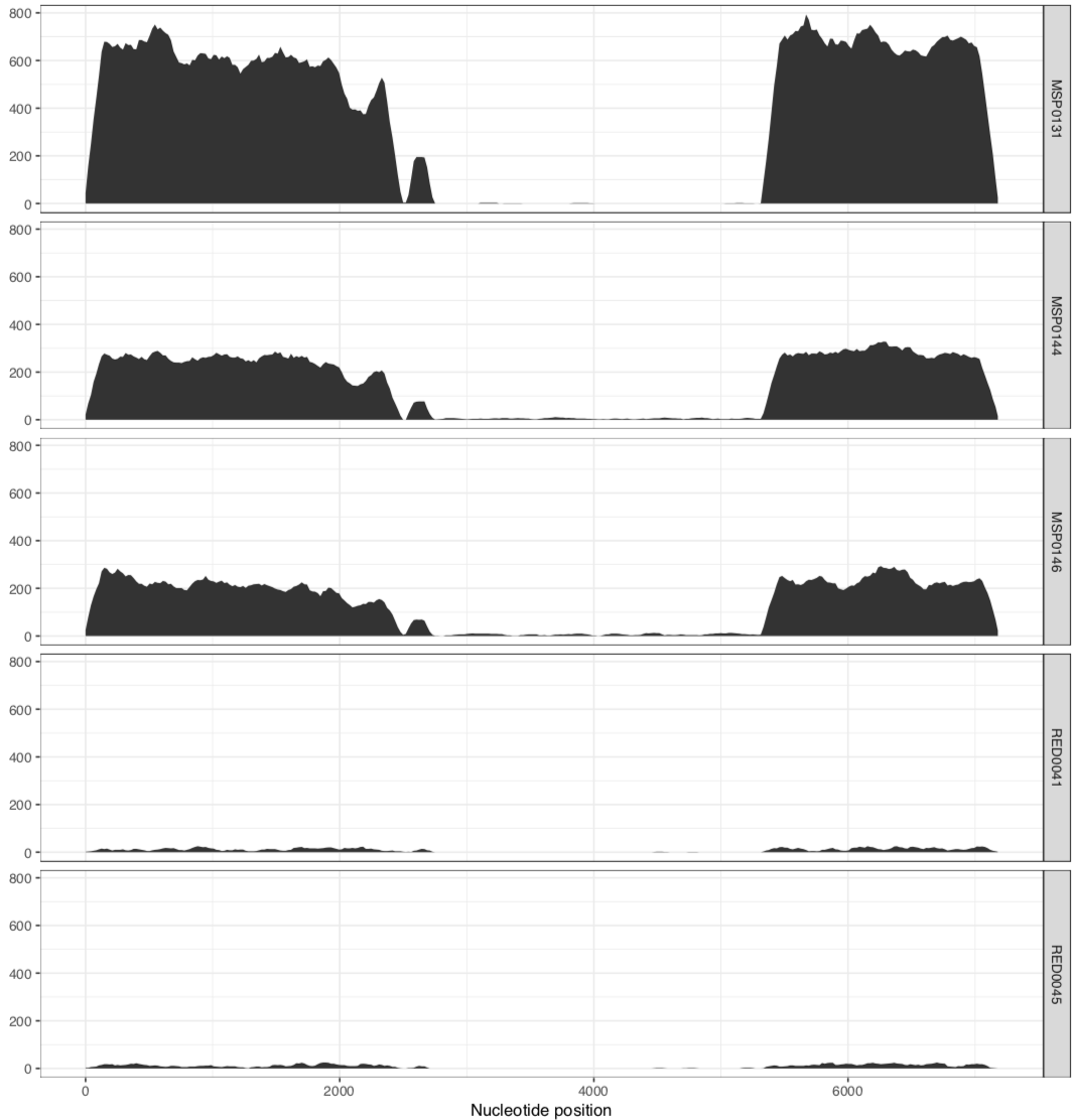
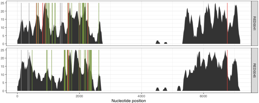
And it would result in two separate PDFs, each with those samples. The first one is the MAL group:
And the other one is the RED group:
Bringing in colors
The outputs above are useful, but they just give you black coverage plots and default SNV colors. Plus, everything has the same y-axis even if the coverage values are radically different. But of course these can be changed to fit the users needs. For example, one can color plots above based on where the samples are from, restrict the maximum coverage to 2000, allow a sliding y-axes for each plot, and have customized SNV lines by running:
anvi-script-visualize-split-coverages -i pLA6_12_000000000001_split_00001_coverage.txt \
                                      -o pLA6_12_000000000001_split_00001_inspect.pdf \
                                      --sample-data sample_data_colors.txt \
                                      --snv-data pLA6_12_000000000001_split_00001_SNVs.txt \
                                      --free-y-scale TRUE \
                                      --max-coverage 2000 \
                                      --snv-marker-transparency 0.9 \
                                      --snv-marker-width 0.1
Where the sample_data_colors.txt file is:
sample_name	sample_group	sample_color
MSP0109	MAL	#000080
MSP0112	MAL	#000080
MSP0114	MAL	#000080
MSP0121	MAL	#000080
MSP0131	MAL	#000080
MSP0144	MAL	#000080
MSP0146	MAL	#000080
RED0041	RED	#8b0000
RED0045	RED	#8b0000
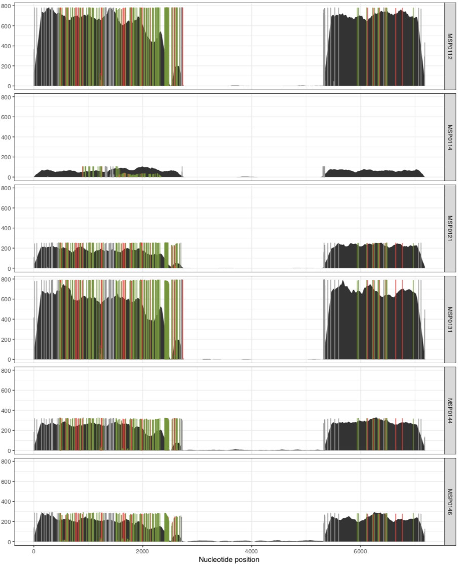
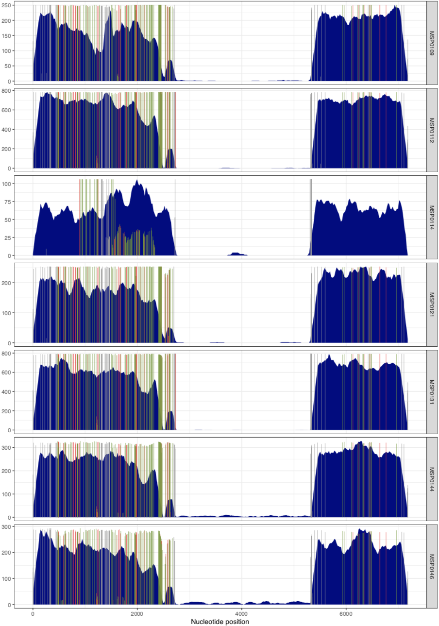
And voila! The MAL group:
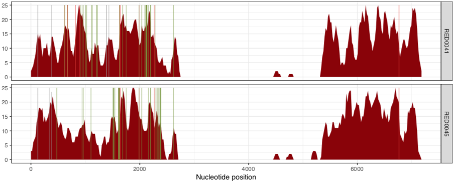
and the RED group:
This is of course just one example of a customizable plot. Please click anvi-script-visualize-split-coverages or use --help in the terminal to see all options available.
Final Words
Now we’ve visualized the mapping results from Petersen et al, we can try to make some fair conclusions.
In their paper, they suggest that this plasmid is nearly identical between all of these metagenomes, aside from the variable region that we can see in the middle. Our mapping results confirm that this is indeed the case. There are a lot of SNVs in comparison to the reference pLA6 12 plasmid, but clearly it is conserved across these environments. However, looking at the coverage plots we can also observe that in samples where there appears to be two versions of the plasmid (e.g., MAP0144 and MSPO0146 where some reads are mapping to the hypervariable region), the SNVs indicate lack of monoclonality in the environment (i.e., they do not extend completely to the top of the plot). This suggests that the version that has the reads mapping to the hypervariable region may also have a slightly different backbone that is more similar to the reference than the rest of the environment.
Thank you very much if you made it all the way to the bottom and if you still have questions about anvi-inspect or anvi-script-visualize-split-coverages feel free to reach out to us.

Happy inspecting!