Ecology of a cryptic plasmid, pBI143


Table of Contents
- Reproducible / Reusable Data Products
- Sequences of the cryptic plasmid pBI143
- Figuring out which version of pBI143 is in a given metagenome
- Characterizing pBI143 biogeography across 100K metagenomes
- The read recruitment from 100K+ metagenomes
- Resolving biome information for metagenomes
- Visualizing pBI143 across biomes and environments
- Additional insights into read recruitment results
- Analyzing mother-infant metagenomes to find evidence for plasmid transfer through single-nucleotide variants (SNVs)
The purpose of this page is to provide access to reproducible data products that underlie our key findings in the study “A highly conserved and globally prevalent cryptic plasmid is among the most numerous mobile genetic elements in the human gut” by Emily Fogarty et al.
If you have any questions and/or if you are unable to find an important piece of information here, please feel free to leave a comment down below, send an e-mail to us, or get in touch with us through Discord:

Reproducible / Reusable Data Products
The following data items are compatible with anvi’o version v7.1 or later. The anvi’o contigs databases and profile databases’ in them can be further analyzed using any program in the anvi’o ecosystem, or they can be used to report summary data in flat-text files to be imported into other analysis environments.
- doi:10.6084/m9.figshare.22308949: Metagenomic read recruitment results from 4,516 global gut metagenomes from healthy individuals using pBI143 Version 1.
- doi:10.6084/m9.figshare.22308964: Metagenomic read recruitment results from 4,516 global gut metagenomes from healthy individuals using pBI143 Version 2.
- doi:10.6084/m9.figshare.22308967: Metagenomic read recruitment results from 4,516 global gut metagenomes from healthy individuals using pBI143 Version 3.
- doi:10.6084/m9.figshare.22308991: Metagenomic read recruitment results from 1,419 gut metagenomes from individuals who were diagnosed with IBD using pBI143 Version 1.
- doi:10.6084/m9.figshare.22309003: Metagenomic read recruitment results from 1,419 gut metagenomes from individuals who were diagnosed with IBD using pBI143 Version 2.
- doi:10.6084/m9.figshare.22309006: Metagenomic read recruitment results from 1,419 gut metagenomes from individuals who were diagnosed with IBD using pBI143 Version 3.
- doi:10.6084/m9.figshare.22309015: Anvi’o single-copy core gene taxonomy for healthy gut metagenomes. Each file in this data pack represents the output of anvi-estimate-scg-taxonomy for a given ribosomal protein run on 3,036 gut metagenomes generated from healthy individuals across the globe.
- doi:10.6084/m9.figshare.22309033: Anvi’o single-copy core gene taxonomy for healthy gut metagenomes. Each file in this data pack represents the output of anvi-estimate-scg-taxonomy for a given ribosomal protein run on on 1,419 gut metagenomes generated from individuals who were diagnosed with IBD.
- doi:10.6084/m9.figshare.22309105: Metagenomic read recruitment results from 936 non-human gut metagenomes using the pBI143 version 1. Metagenomes used for this analysis include open and coastal marine metagenomes from the Tara Oceans and Ocean Sampling Day projects, human oral and skin metagenomes from the Human Microbiota Project, primate gut metagenomes, dog metagenomes, and sewage metagenomes around the globe. Their accession numbers are available via the Supplementary Table 1 (alternative_environment tab) of the study.
- doi:10.6084/m9.figshare.22309114: Metagenomic read recruitment results from 4,516 global gut metagenomes from healthy individuals using the crAssphage genome.
- doi:10.6084/m9.figshare.22298215: Metagenomic read recruitment results from four mother-infant datasets from Finland, Italy, Sweden, and the United States. These data enabled us to study the population genetics of pBI143 in mothers and their infants to establish an understanding of the vertical transmission of the cryptic plasmid. A reproducible bioinformatics workflow for the analysis that rely upon these files is below.
- doi:10.6084/m9.figshare.22336666: Supplementary Tables and Supplementary Information files.
Sequences of the cryptic plasmid pBI143
In our study we identified three sequence-discreet version of pBI143 across human gut metagenomes. We used all three versions extensively for our analyses, and the summary figure below shows the distribution of the pBI143 and its versions across the globe:
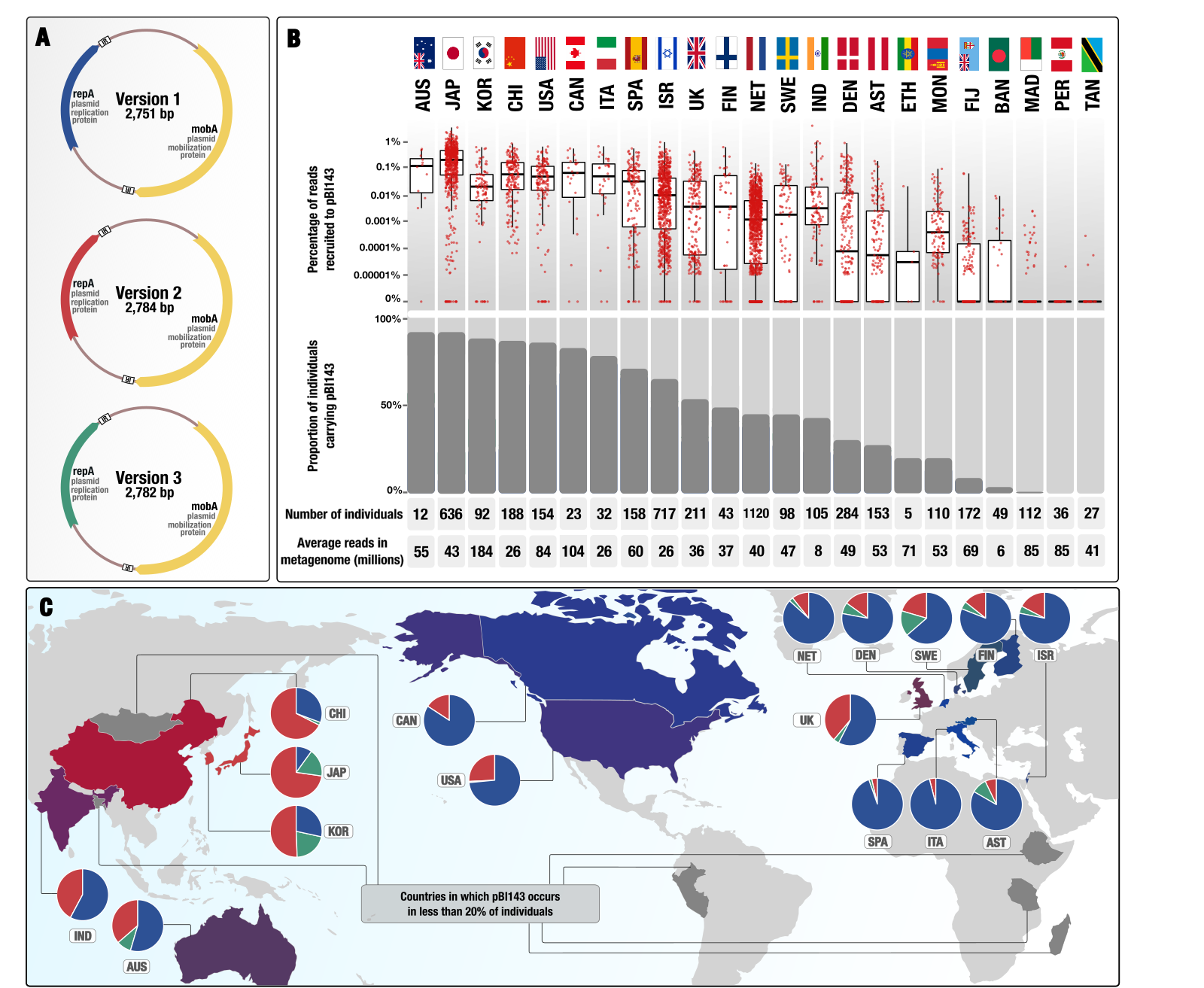
The draft Figure 1 from our study that depicts pBI143 prevalence and abundance in globally distributed human populations.
pBI143 Version 1
Assembled from a metagenome internally labeled as USA0006 (NCBI accession: SRX023606):
>pBI143_V1
AAAGCCGCTGGAGATGTCGGATGTCCGTCAATTAACTCCAGCGGCTTGTATTTTGGTAACTCTCCCGTATCGGTCGGCTA
CCGTTTGGTCAGCAACAAAGGTAGTACTTTATTGTCGCAAATCCAAATGTTTTCCCCTTTATTTGTGCATTTACAGAACA
TTTGCTAACTTCGCACCTATGCAGTATGGTGATAGCACACTAGCACCCTAAAGGGTGCGTGTGTAAGGGGACAAGCCCCC
TTAACCCCCTGTCAGCCGGCTGTCACCGGCTGTTATCGATTGTCACAAAAATGTTAACTTATGGGAGCAACAAGTATTCA
TGTACAAGCAGTGAAGCCGGGGAGTGAGATTCACAACTTTAGGGAAAAAGAGTTGGACTATGTTCGTCCCGAACTTAGTC
ATTTGAATGAAAGCTGGGTTGGAGATAGCATCTCCCATCGGCTGGAAAGTGCGAAACAAAGATATCTCGATACGGTTGGG
CAGAAGATGCAGGCTAAAGCCGCACCCATACGAGAGGGAGTAATAGTAATCAAACAAGAAACCACCATGCAGGAACTCCA
GCAGTTTGCCACGGTCTGCAAAGAACGTTTCGGTATCGAAGCATTTCAAATCCATATACACAAGGACGAAGGATACATGA
ACGCAAAGCAATGGACACCTAACCTTCATGCCCATGTAGTTTTCGATTGGACGCAGCCGAATGGGAAAAGTGTGCGTTTA
TCGCGTGATGACATGGCAGAACTCCAAACCATAGCATCTGAAACACTGGGCATGGAACGTGGCGTTTCTTCTGACCGCAA
ACACTTATCGGCTATGCAGTACAAGACCGAATGTGCGAAAGAACAGCTTCAGGAACTATCAAACGATATATCCAGTGCAT
TAGACAAACACAAGGACGTACAAAACCAGCTTCTTCAGCTTCAGAAAGAACTACGTTCCATTGAAACAAAGAAGAACGTC
CAAAAACTCATTTCTAAGGCTTCAGAGAAGTTTTACGGCTTGATTGGAAAAACAGTCAACGATAGGGAAAAGGATGCCTT
AAAAGCCAAAGTAAAGGCTTTAGAGGGGGAAAATGAACAGCTATCCGATAGACTGGGAAAGGCTATACTTGAAAAAGAGC
AAAACGGCACAAAGGCATTCAAAGCCGAGAATGACAAGGAGTATTATAGACAACAAATGGACAACGCAAGGACAACCAGT
AACCGATTAAGGACGGAGAACCAAGAACTAAAGACCGAAACCAAGGAATTGAAAAAAGAACTTGGTAAGATGAAAGACTT
GTTCAATTCCGAACAACTGGAGGCTTTAAGGCATCATTTCCCAAACATATCAAAAGCTATGGAAGAGGGGAAAGACCTAC
TCAAGCAAATCACCAGAAGCAGAGGTTTCGGTATGGGTATGTAACCCCCCCCCGCCCCCAAAGGGGGAGCGACCAAACGG
CAGCCTCTCTCAATGGAGTGTTACGTCGTTCGGATTCGGAAGAAATTTTGCAGGGTTCGGAAAACGGTTGTGTGCTTATT
CTAAAAAAAGTTTATGGTGTGGCGCTCGTCGGGACGGGTGGTCCCGCCCCTTGCCGCTGGGCGCTCCCCGACCGATGATT
TTTAAGTGACTGATTTTGTGCTGTTTTGGGGGTATATTAAGAATAGAAGAAATAGAATAAGTTAAGTACTTGATACACAA
TATAGGGCATTTTCCATATTGGAAATTCTCATTTTCCAATCTAGAAAATACTGATTTCCTAATATAATACTAAACAGGAA
AATAATATTTCCCTTAATATTGTTTTTATGGAAAATAATAGTTTACTTTGTGGAGAATAATATTTCCCAAAAACACATCA
AAATGGAAAATAAAAAAGCAGTTAAGTTAACCGATTTTCAAAAGAACGAAGAAAATCCTTTTATGAAACAAGCTATAGAA
GGTATTGAAAATCATGTTGTTAAAAAGTATAAGAGTAATAGTGGTGGCGATAAGAGAGCCGTAGTAGCTTTAGCCGACAC
TGAAACTGGAGAAGTGTTTAAGACTTCGTTTATCCGTCAAATAGAAGTAGATGAAGAACAATTCACTAAATTGTATCTTT
CTAACTTTGCTGCATTCTTTGACCTATCACAAGCAGCTATTCGGGTTTTTGGTTACTTTATGACCTGCATGAAACCCAAA
AATGATTTAATCATCTTCAATAGAAAAAAATGCCTAGAATATACCAAATACAAAACAGACAAAGCCGTTTATAAAGGACT
TGCAGAACTTGTAAAAGCTGAAATCATAGCCCGAGGACCAGCCGATAATCTTTGGTTTATTAATCCTCTGATAGTATTCA
ATGGTGACCGAGTGACATTTGCTAAAACATACGTTCGGAAAAAGACTTTAGCTGCCCAAAAGAAAGAAGAAGCAGAGAAA
CGACAATTATCACTTGGCTTTGATGAACAGTAACACTCCATTGAGTGAAGCTGCCGTTTGGTCGCTCCCCCTTTGGGGGC
GGGGGGGGGATAGATAAAGTTCCTCTATGTAAAGTTATAATGGGGGATGAAAGGCAAGGTTCGCTAACCTTACCCCGATT
GTTTATGCTTCCCAGCATTCAATCTATCCCCGTTTATGGGTTTCTCTTTCACCCTACAAAGATAACCTCATGGGGGAAAA
ATGTCCAAGAATATGGGGTAAAAACTATCAAGTCGGTAGAAAATAAGTATCTTTGAAGTACATTTTTAGTAGAGGTACTG
GTATGCCTAGACGAAGCAGATAGGCAAAAAT
pBI143 Version 2
Assembled from a metagenome internally labeled as CHI0054 (NCBI accession: SRR341705):
>pBI143_V2
AAAGCCGCTGGGGATGTCGGATGTCCGTCAATTAACTCCAGCGGCTTGTATTTTGGTAACTCTCCCGTATCGGTCAGCTA
CCGTTTGGTCAGCAACAAAGGTAGTACTTTATTGTCGCAAATCCAAATGTTTTCCCCTTTATTTGTGCATTTACAAAACA
TTCACTAACTTCGCACCTATGCAGTATGGTGATAGCACACTAGCACCCTAAAGGGTACGTGTGTAAGGGGACAAGCCCCC
TTAACCCCCTGTCAGCCGGCTGTCACCGGCTGTTATCGATTGTCACAAAAATGTTAACTTATGGGAGCAACAAGTATTCA
TGTACAAGCAGTGAAGCCGGGGAGCGAGATTCACAACTTTAGGGAAAAAGAGTTGGACTATGTTCGTCCGGAACTTAGTC
ATTTGAATGAAAGCTGGGTTGGAGATAGCATCTCCCATCGGCTGGAGAGTGCGAAACAGAGATATTTCGATACGGTTGGG
CAGAAGATGCAGACTAAAGCAGCACCCATACGGGAGGGGGTAATAGTAATCAAGCAAGAAACCACCATGCAGGAACTCCA
GCAATTCGCTGCGGTCTGCAAGGAACGTTTCGGTATTGAAGCGTTTCAAATCCATATACACAAGGACGAAGGATACATGA
ACGCAAAGCAATGGACACCTAACCTTCACGCCCATGTAGTTTTCGATTGGACGCAGCCGAACGGGAAGAGTGTGCGTTTA
TCGCGTGATGACATGGCAGAACTCCAAACCATAGCATCTGAAGCACTGGGCATGGAACGTGGTGTTTCTTCTGATCGCAA
ACACTTATCGGCTATGCAGTACAAGACCGAATGTGCGAAAGAACAGCTTCAGGAACTATCCAACGATATATCCAGTGCGT
TAGACAAGCACAAGGACGTGCAAAACCAGCTTCTTCAGCTTCAGAAAGAACTACGTTCCATTGAAACAAAGAAAAACGTC
CAAAAACTCATTTCTAAGGCTTCAGAGAAGTTTTACGGCTTGATAGGGAAAACGGTTAACGATAGGGAAAAAGATGCCTT
AAAAGCCAAAATAAAGGCTTTAGAGGGGGAAAATGAACAGCTATCCGATAGACTGGGAAAGGCTATACTTGAAAAAGAGC
GAAACGGCACAAAGGTATTCAAAGCCGAGAACGACAAGGAGTATTATAGACAGCAAATGGACAATGCAAGGACAACCAGT
AACCGACTAAGAACGGAGAACCAAGAACTAAAGACCGAAACCAAGGAATTGAAAAAAGAACTTGGTAAGATGAAAGACTT
GTTCAATTCCGAACAACTGGAGGCTTTAAGGCATCATTTCCCAAACATATCAAAAGCTATGGAAGAGGGGAAAGACCTAC
TCAAGCAAATCACCAGAAGCAGAGGTTTCGGCATGGGTATGTAACCCCCCCCCGCCCCCAAAGGGGGAGCGACCAAACGG
CAGCTTCACTCAATGGAGTGTTACGCCGTTCGGGTTCGGAAGAAATTTTGCAGGGTTCGAAAAACGGTTGTGTGCTTATT
CGAAAAAAAGTTTATGGTGTGGGCGCTCGTCGGGACGGGTGGTCCCGCCCCTTGCCGCTGGGCGCTCCCCGACCGATGAT
TTTTTAAGTAGTTGATTATATGCCGTTTTTAGGGTATAATAAGAACTTAAGAAATAGAATAAGTTAAGTAGTTGATACTC
AATATAGGGTATTTTCCATATTGGAAAATCTGATTTTCCATATTAGAAAGTCACTCTTTCCTATTAGATGTTAAAAAGGA
AAATATATTTTGCTTTTTTATTGTATTAATGGAAATTTAAATATTCCTTTGTGGAAAATCAAATTATACTTTTTCACCGA
TATATAGAAAGTCAAATTTGCCTAAATAGAATGTTTATGGAAAATAAGAAAGTACTCAAATTAACCGATTTTCAAAAAAA
CGAAGAAAACCCCTTTATGAAACAAGCAATTGAAGGGATTGAAAATCACGTTGTTAAGAAATACAAAAGTAGTACGGGAA
GTGATAAAAAAGCTGTAGTTGCTGTTGCTGATACAGATACAGGAGAAGTATTCAAAACCTCGTTTATCCGACAAATAGAA
GTAGATGAAGAGCAATTTGCAAAACTATACCTTGCGAATTTTGCCGCTTTTTTCAATCTATCACAATCAGCTATTCGGGT
TTTCGGGTATATTCTAACTTGCATGAAGCCTAAGAATGATATGATAATTTTCGATAGGCGAAAATGCTTAGAATACACCC
AATACAAATCAGACAAAGCCATATACAAAGGATTGGCAGAGCTCGTACAAAGTGAAATCATAGCAAGAGGTCCAAACGAA
TATAATTGGTTCATTAATCCGTTGATTGTCTTTAATGGGGATAGGGTTTCATTTACAAAAACATACGTTCGGAAAAAGAC
TTTAGCTGCCCAAAAGAAAGAAGAAGCAGAGAAACGACAGTTATCACTTGGTTTTGATGAACTGTAACACTCCATTGAGT
GAAGCTGCCGTTTGGTCGCTCCCCCTTTGGGGGCGGGGGGGGATAGATAAAGTTCCTCTATGTAAAGTTATAATGGGGGA
TGAAAGGCAAGGTTCGCTAACCTTACCCCGATAGTTTATGCTTCCCAGCATTCAATCTATCCCCGTTTATGGGTTTCTCT
TTCACCCTACAAAGATAACCTCATGGGGGAAAAATGTCCAAGAATATGGGGTAAAAACTATCAAGTCGGTAGAAAATAAG
TATCTTTGAAGTACATTTTTAGTAGAGGTACTGGTATGCCTAGACGAAGCAGATAGGCAAAAAT
pBI143 Version 3
Assembled from a metagenome internally labeled as ISR0084 (NCBI accession: ERR1136776):
>pBI143_V3
AAAGCCGCTGGAGATGTCGGATATCCGTCAATTAACTCCAGCGGCTTGTATTTTGGTAACTCTCCCGTATCGGTCAGCTA
CCGTTTGGTCAGCAACAAAGGTAATGCTTTATCATCGCAATTCCAAATGTTTTTCCCTTTATTTGTGCATTTACAAAACA
TTCACTAACTTCGCACCTATGCAGTATGGTGATAGCGCACTAGCACCCTAAAGGGTGCGTGTGTAAGGGGACAAGCCCCC
TTAACCCCCTGTCAGCCGGCTGTCACCGGCTGTTATCGATTGTCACAAAATGTTAACTTATGGGAGCAACAAGTATTCAT
GTACAAGCAGTGAAGCCGGGGAGCGAGATTCACAACTTTAGGGAAAAAGAGTTGGACTATGTTCGTCCGGAACTTAGTCA
TTTGAATGAAAGCTGGGTTGGAGATAGCATCTCCCATCGGCTGGAGAGTGCGAAACAGAGATATTTCGATACGGTTGGGC
AGAAGATGCAGACTAAAGCAGCACCCATACGGGAGGGGGTAATAGTAATCAAGCAAGAAACCACCATGCAGGAACTCCAG
CAATTCGCTGCGGTCTGCAAGGAACGTTTCGGTATTGAAGCGTTTCAAATCCATATACACAAGGACGAAGGATACATGAA
CGCAAAGCAATGGACACCTAACCTTCACGCCCATGTAGTTTTCGATTGGACGCAGCCGAACGGGAAGAGTGTGCGCTTAT
CGCGTGATGACATGGCAGAACTCCAAACCATAGCATCTGAAGCACTGGGCATGGAACGTGGTGTTTCTTCTGACCGCAAA
CACTTATCGGCTATGCAGTACAAGACCGAATGTGCGAAAGAACAGCTTCAGGAACTATCCAACGATATATCCAGTGCGTT
AGACAAGCACAAGGACGTGCAAAACCAGCTTCTTCAGCTTCAGAAAGAACTACGTTCCATTGAAACAAAGAAAAACGTCC
AAAAACTCATTTCTAAGGCTTCAGAGAAGTTTTACGGCTTGATAGGGAAAACGGTTAACGATAGGGAAAAAGATGCCTTA
AAAGCCAAAATAAAGGCTTTAGAGGGGGAAAATGAACAGCTATCCGATAGACTGGGAAAGGCTATACTTGAAAAAGAGCG
AAACGGCACAAAGGTATTCAAAGCCGAGAACGACAAAGAGTATTATAGACAGCAAATGGACAATGCAAGGACAACCAGTA
ACCGACTAAGAACGGAGAACCAAGAACTAAAGACCGAAACCAAGGAATTGAAAAAAGAACTTGGTAAAATGAAAGACTTG
TTCAATTCCGAACAACTGGAGACTTTAAGACATCATTTCCCGAACATATCGAAAGCTATGGAAGAGGGGAAAGACCTACT
CAAGCAAATCACCAAAAGCAGGGGTTTCGGCATGGGTATGTAACCCCCCCCGCCCCCAAAGGGGGAGCGACCAAACGGCA
GCTTCACTCAATGGAGTGTTACGCCGTTCGGATTCAGAAACTTCACTCAATGGAGTGTTACGCCGTTCGGATTCAGAAAA
CATTTTGCAGGGTTCGAAAAACGGTTGTGTGCTTATCCGAAAAAAAGTTTATGGTGTGGGCGCTCGTCGGGACGGGTGGT
CCCGCCCCTTGCCGCTGGGCGCTCCCCGACCGATGATTTTTAAGTGGCTGATTTTGTGCTGTTTTGGGGGTGTATTAAGA
ACTATAAGAAACAACATAAGCTAAGTAATTGATAATCAATATAGGCTAGTTCACACTGTATGAACTGCCAGTTCAATCTA
GCTTGAACTCAGAGTTCAATAAATCATGTTAAAAATCGAACTGTGTGTTTATTTTTGTTGGACTGATAGTCTATATTTGT
AGGCGAAAAATCGAACTAATAGAATAATATACCATGGCAAAAAACGAACTAAAATTATCCGACTTCCAAAGGAATAAGGA
AAATCCATTCATGAAGCAAGCAATAGAAGATATTGAAAATCATGTTGTTAAAAAATATAAGAGCAGTACAGGAAGTGACA
AAAAAGCAGTTGTTGCCGTTGCTGATACAGATACAGGAGAAGTGTTCCGAACTTCCTTTATTCGACAGATAGAAGTAGAT
GAAGAACAATTTGCAAAACTCTATCTGAACAATTTTGCTGCATTTTTTGACCTTTCACAAGCCGCAATAAGGGTATTTGG
CTATATCATGACTTGTATGAAACCCAAGAATGATATGATAATGTTTATCCTAGAAGATTGTCTTGAATATACGAAATATA
CAAGCAAAGGTACAGTTTATCGAGGGCTTGCAGAACTGGTTAAAGCGGAGATTATAGCCAGAGGTATAAACGAGAACTTA
TGGTTCATCAATCCCCTTATAGTTTTCAATGGGGATAGAGTTTCTTTTACCAAAACATACGTTCGGAAAAAATCTCTATC
AACTAAAAAGAAAGCTGAAGAAGATGAACGCCAGCTATCTTTAGGTTTCAGTTCAGAGTAACACTCCATTGAGCGAAGCT
GCCGTTTGGTCGCTTCCCCCCTTGGGGGACGGGAGGGGGATAGGATAAAGTTCCTCTATGTAAAGTTATAATGGGGGATA
AAGGCAAGGTTCGCTAACCTTACCCCGATTGTCTATGCTTCCCAGCATCCAATCTACCCCCGTTTATGGGTTTCTCTTTC
ACTTTACAAAGATAACCTCATGGGGGAAAAATGTCCAAGAATATGGGGGAAAATCTATCAAATCAGTAGAAAATTAGTAT
CTTTGGGGGACACTTCTAATGGGGGTACTGGTATAGCCTAGACGAAGCGGATAGGCGAAAAT
Figuring out which version of pBI143 is in a given metagenome
To precisely identify which version of pBI143 is in a given metagenome, we implemented a Python program that would consider coverage ratios between mobA and repA genes based on metagenomic read recruitment results for each version of the plasmid.
The following steps describe our workflow that resulted in the determination of the appropriate version of pBI143 in a given metagenome:
- Recruit reads from your metagenome,
M, using each version of pBI143,v1,v2,v3, separately. - Profile resulting BAM files using anvi-profile.
- Export nucleotide-level coverage data from each profile database using the program anvi-get-split-coverages to get individual coverage profiles,
M_v1,M_v2,M_v3. - Then run the Python program choose-plasmid-version-based-on-coverage-ratios.py the following way:
python choose-plasmid-version-based-on-coverage-ratios.py M_v1 M_v2 M_v3
This will generate a 2-column TAB-delimted file called ALTERNATIVES.txt in your work directory, where each line will represent a metagenome M and which version of the plasmid is the version it contains (e.g., M_v3), if the metagenome does contain pBI143 and if the version could be resolved confidently. Instances where a robust conclusion could not be made by the program will be clearly marked in the output file as well. For posterity, this is the source code for choose-plasmid-version-based-on-coverage-ratios.py:
#!/usr/bin/env python
# -*- coding: utf-8

import sys
import argparse
import numpy as np

from itertools import chain
from collections import Counter

import anvio.utils as utils
import anvio.filesnpaths as filesnpaths

from anvio.errors import ConfigError, FilesNPathsError

regions_of_interests = {'repA': (1809, 2467), 'mobA': (300, 1404)}
min_avearge_coverage = 1

def main(args):
    input_file_paths = args.input_files

    regions_max = max([max(e) for e in regions_of_interests.values()])
    regions_min = min([min(e) for e in regions_of_interests.values()])

    d = {}
    for input_file_path in input_file_paths:
        filesnpaths.is_file_exists(input_file_path)
        filesnpaths.is_file_tab_delimited(input_file_path, expected_number_of_fields=5)

        # alternative input to consider. will appear in `d` later:
        alt = input_file_path.split('.txt')[0]

        contents_dict = utils.get_TAB_delimited_file_as_dictionary(input_file_path)

        for e in contents_dict.values():
            pos = int(e['nt_position'])
            if pos > regions_min and pos < regions_max:
                # this is within the min/max range of thins we are interested but
                # we are not sure if it is relevant yet
                for region in regions_of_interests:
                    if pos > min(regions_of_interests[region]) and pos < max(regions_of_interests[region]):
                        # we are in 'region'
                        sample = e['sample_name']

                        if sample not in d:
                            d[sample] = {}

                        if alt not in d[sample]:
                            d[sample][alt] = {}

                        if region not in d[sample][alt]:
                            d[sample][alt][region] = []

                        d[sample][alt][region].append(int(e['coverage']))
                    else:
                        continue

    alternatives = {}
    mean_coverages = {}
    for sample in d:
        mean_coverages[sample] = Counter()
        for alt in d[sample]:

            # store the average coverage of all regions for the alternative
            mean_coverages[sample][alt] = np.mean(list(chain(*d[sample][alt].values())))

            for region in d[sample][alt]:
                d[sample][alt][region] = {'cov': np.mean(d[sample][alt][region]), 'det': len([p for p in d[sample][alt][region] if p > 1]) / len(d[sample][alt][region])}


        # remove alternatives if they don't have prper mean coverage
        alternatives_to_remove_due_to_min_coverage = [alt for alt in mean_coverages[sample] if mean_coverages[sample][alt] < min_avearge_coverage]
        for alt in alternatives_to_remove_due_to_min_coverage:
            d[sample].pop(alt)

        if not len(d[sample]):
            alternatives[sample] = {'plasmid_version': 'NONE_DUE_TO_MIN_COVERAGE'}
            continue

        regions_for_consideration = []
        # first check for detection. if any of regions of interest has detection less than 1.0,
        # they are out of consideration:
        for alt in d[sample]:
            if len([r for r in d[sample][alt] if d[sample][alt][r]['det'] > 0.9]) == len(regions_of_interests):
                regions_for_consideration.append(region)

        if not len(regions_for_consideration):
            alternatives[sample] = {'plasmid_version': 'NONE_DUE_TO_NO_REG_DETECTION'}
            continue

        # for the remaining ones, we want to compare the ratio between alternatives
        for alt in d[sample]:
            d[sample][alt]['ratios'] = d[sample][alt]['mobA']['cov'] / d[sample][alt]['repA']['cov']

        ratios = [(alt, d[sample][alt]['ratios']) for alt in d[sample]]
        ratios_within_range = [(r[0], abs(1 - r[1])) for r in ratios if r[1] > 0.1 and r[1] < 4]

        if not len(ratios_within_range):
            alternatives[sample] = {'plasmid_version': 'NONE_DUE_TO_BAD_RATIOS'}
            continue

        # alternative version of the plasmid for this metagenome is determined here:
        alternative = sorted(ratios_within_range, key = lambda x: x[1])[0][0]
        alternatives[sample] = {'plasmid_version': alternative}

    utils.store_dict_as_TAB_delimited_file(alternatives, 'ALTERNATIVES.txt', headers=['metagenome', 'plasmid_version'])


if __name__ == '__main__':
    parser = argparse.ArgumentParser(description='Process multiple split nt coverages files')

    parser.add_argument('input_files', metavar = 'SPLIT_NT_COVERAGE_FILES', nargs='+',
                        help = "Split nt coverages to process")

    args = parser.parse_args()

    try:
        main(args)
    except ConfigError as e:
        print(e)
        sys.exit(-1)
    except FilesNPathsError as e:
        print(e)
        sys.exit(-1)
Characterizing pBI143 biogeography across 100K metagenomes
Our initial investigations of the distribution of pBI143 indicated that this cryptic plasmid is largely exclusive to the human gut environment, and it did not occur in terrestrial, marine, or other host-associated habitats except cats (really – it was absent everywhere, including dogs or cows or sheep, but our PCR assays did detect pBI143 in cats, more on this later).
To quantify the ecology of pBI143 much more broadly, we performed a large-scale read recruitment analysis for pBI143 across over 100,000 metagenomes and quantified its distribution patterns across a very large number of habitats. This investigation was consisted of multiple steps, including,
- Using all three versions of the pBI143 to recruit reads from a collection of 100,000+ metagenomes and profiling the resulting BAM files.
- Resolving the biome information for each metagenome and identifying which pBI143 version best represents the pBI143 population found in each metagenome.
- Visualizing pBI143 detection patterns across biomes and environments.
The following sections detail each step, followed by a brief discussion over these results, in addition to those that appear in our paper.
The read recruitment from 100K+ metagenomes
The anvi’o program anvi-profile-blitz profiled the BAM files samtools generated from Bowtie2 read recruitment results to report the distribution patterns of all three versions of pBI143 across all metagenomes. anvi-profile-blitz reports a detailed output for read recruitment statistics, called bam-stats-txt, and you can see the standard headers in the output by visiting the artifact page.
The raw output file from anvi-profile-blitz is available here: anvi-profile-blitz.txt.gz
Resolving biome information for metagenomes
Accurate determination of the ecology of pBI143 through metagenomic read recruitment requires accurate insights into the origin of each metagenome used in such an analysis. Which is quite a significant challenge since the metadata associated with metagenomes stored on the NCBI can be misleading or insufficient. For instance, the biome information for all metagenomes in a single project that includes gut metagenomes from multiple animal species may simply be called ‘gut metagenome’, or the biome information for a project that includes marine sediment metagenomes may simply be set as ‘metagenome’.
To maximize the accuracy of our investigation, we first identified all ambiguous cases (where the biome information for the NCBI BioProjects were ‘metagenome’, ‘gut metagenome’, ‘human metagenome’) and then we revisited the publications in which these datasets were generated to manually assign a more specific biome information to these datasets. We documented our efforts in the following Python program, which generated an updated bam-stats-txt file with the additional columns, including biome, for downstream visualization tasks.
The final output file generated by this program is available here: read-recruitment-results.txt.gz
#!/usr/bin/env python
# We used this Python script to generate a final output file for the metagenomics read
# recruitment statistics of the pBI143 from various 'biomes'. The script takes in
# various files that describe metagenomes or the profiling of BAM files after the read
# recruitment was completed and merges them while improving the 'biome' information for
# each metagenome using dictionaries we have prepared manually. the resulting file
# is used to quantify pBI143 distribution across biomes inside and outside of human
# habitats in Fogarty et al.
import sys
from anvio.utils import get_TAB_delimited_file_as_dictionary, store_dict_as_TAB_delimited_file
# metadata file that contains additional information for each metagenome per accession id
sample_metadata = get_TAB_delimited_file_as_dictionary("sample-metadata.txt")
# metadata file that shows the total number of reads per metagenome, with column
# names `SAMPLE`, `READS`, `BASES`, `INSERTS`.
sample_read_counts = get_TAB_delimited_file_as_dictionary("sample-read-counts.txt")
# the raw output file generated by `anvi-profile-blitz` from the BAM files where each three
# version of the pBI143 was used to recruit reads independently from each metagenome listed
# in `sample-metadata.txt` file.
anvi_profile_blitz_results = get_TAB_delimited_file_as_dictionary("anvi-profile-blitz.txt",
indexing_field=-1)
###########################################################################################
# The information in the following sections of the code evolved over time. We updated these
# dictionaries to associate individual metagenomes with individual 'biomes' as we manually
# investigated each publication associated with each dataset to recover a more accurate
# biome information especially for datasets where their biome information was officially
# listed as `metagenome` or `human metagenome`.
###########################################################################################
specific_scientific_names_for_bioprojets = {'PRJNA781406': 'water/sediment metagenome',
'PRJNA682246': 'human gut metagenome',
'PRJEB14050': 'human-associated bacterial culture wgs',
'PRJNA338184': 'human-associated bacterial culture wgs',
'PRJNA724996': 'marine sediment metagenome',
'PRJNA623111': 'marine sediment metagenome',
'PRJEB7866;': 'hydrothermal vent metagenome',
'PRJEB19456;': 'hydrothermal vent metagenome',
'PRJNA846291;': 'human airway-associated metagenome',
'PRJNA595703': 'human airway-associated metagenome',
'PRJEB45443': 'infant gut metagenome',
'PRJEB32631': 'infant gut metagenome', # actually only largely infant. includes mothers. ceserian vs natural birth
'PRJNA475246': 'infant gut metagenome', # actually only largely infant. assholes didn't report anything in metadata.
'PRJNA376566': 'infant gut metagenome',
'PRJEB13870': 'human gut metagenome',
'PRJEB23561': 'cow rumen metagenome',
'PRJEB21624': 'cow rumen metagenome',
'PRJEB10338': 'cow rumen metagenome',
'PRJNA813429': 'glacier metagenome',
'PRJNA715601': 'infant gut metagenome',
'PRJNA695070': 'infant gut metagenome',
'PRJEB39306': 'urban water/sediment metagenome',
'PRJNA437202': 'coral metagenome',
'PRJEB18063': 'lake water/sediment metagenome',
'PRJEB6337': 'human gut metagenome',
'PRJEB31632': 'hospital surfaces',
'PRJNA685797': 'human gut metagenome',
'PRJNA714147': 'wastewater metagenome',
'PRJEB38662': 'marine metagenome',
'PRJNA629517': 'marine metagenome',
'PRJNA274897': 'marine metagenome',
'PRJEB15043': 'marine metagenome',
'PRJNA504891': 'human gut metagenome',
'PRJNA529124': 'human gut metagenome',
'PRJNA529400': 'human gut metagenome',
'PRJEB22893': 'human gut metagenome',
'PRJNA491335': 'human gut metagenome',
'PRJNA723432': 'goat gut metagenome',
'PRJEB49383': 'infant gut metagenome',
'PRJEB39610': 'infant gut metagenome',
'PRJNA630999': 'infant gut metagenome',
'PRJNA301903': 'infant gut metagenome',
'PRJNA294605': 'infant gut metagenome',
'PRJNA273761': 'infant gut metagenome',
'PRJNA327106': 'infant gut metagenome',
'PRJNA473126': 'infant gut metagenome',
'PRJNA396794': 'infant gut metagenome',
'PRJNA489090': 'infant gut metagenome',
'PRJNA649484': 'rRNA amplicons',
'PRJNA485056': 'human gut metagenome',
'PRJNA361402': 'human gut metagenome',
'PRJNA352220': 'human gut metagenome',
'RJEB22893': 'human gut metagenome',
'PRJEB17632': 'human gut metagenome',
'PRJNA438384': 'marine biofilm metagenome',
'PRJEB56022': 'human gut metagenome',
'PRJNA375935': 'human gut metagenome',
'PRJEB6070': 'human gut metagenome',
'PRJNA389927': 'human gut metagenome',
'PRJNA449784': 'human gut metagenome',
'PRJEB9150': 'human gut metagenome',
'PRJNA613947': 'human gut metagenome',
'PRJNA915251': 'human gut metagenome',
'PRJNA763692': 'human gut metagenome',
'PRJEB30834': 'human gut metagenome',
'PRJEB26961': 'pig gut metagenome',
'PRJEB34871': 'human gut metagenome',
'PRJEB20308': 'dog gut metagenome',
'PRJNA217052': 'human gut metagenome',
'PRJEB27308': 'human gut metagenome',
'PRJEB1775': 'human gut metagenome',
'PRJNA420682': 'bovine gut metagenome',
'PRJEB32731': 'human gut metagenome',
'PRJEB1786': 'human gut metagenome',
'PRJNA698754': 'seawall biofilm metagenome',
'PRJEB14847': 'human gut metagenome',
'WASABI': 'urban environment metagenome',
'Zenodo': 'various wild animals',
'PRJEB40256': 'human gut metagenome',
'PRJNA379120': 'human gut metagenome',
'PRJEB24041': 'human gut metagenome',
'PRJEB40628': 'human gut metagenome',
'PRJEB9357': 'cat gut metagenome',
'PRJEB33338': 'chicken gut metagenome',
'PRJEB38174': 'chicken gut metagenome',
'PRJEB39057': 'zebu gut metagenome',
'PRJEB8094': 'human gut metagenome',
'PRJNA656389': 'buffalo gut metagenome',
'PRJEB31971': 'ancient human remains',
'PRJEB19857': 'human gut metagenome',
'PRJEB39223': 'human gut metagenome',
'PRJNA399742': 'human gut metagenome',
'PRJEB28237': 'human gut metagenome', # this includes also culture-enriched microbiota metagenomes :/
'PRJEB22973': 'laboratory rat gut metagenome',
'PRJEB42363': 'infant gut metagenome',
'PRJNA686265': 'human gut metagenome',
'PRJEB28097': 'human gut metagenome',
'PRJEB38669;PRJEB44815': 'marine metagenome'
}
###########################################################################################
# Simpler names for scientific species names used in the 'host name' column in the
# metagenome metadata.
###########################################################################################
specific_scientific_names_for_host_names = {'sus scrofa': 'wild boar gut metagenome',
'bos taurus': 'cow gut metagenome',
'gallus gallus': 'chicken gut metagenome',
'balaenoptera physalus': 'whale gut metagenome',
'megaptera novaeangliae': 'whale gut metagenome',
'eubalaena glacialis': 'whale gut metagenome',
'balaenoptera borealis': 'whale gut metagenome',
'numida meleagris': 'fowl gut metagenome',
'bubalus bubalis': 'buffalo gut metagenome',
'water buffalo': 'buffalo gut metagenome',
'dairy cattle': 'cow gut metagenome',
'goat': 'goat gut metagenome',
'grazing goat': 'goat gut metagenome',
'guangxi goat': 'goat gut metagenome',
'hainan goat': 'goat gut metagenome',
'newborn goat': 'goat gut metagenome',
'sichuan goat': 'goat gut metagenome',
'myodes glareolus': 'mouse gut metagenome',
'ovis aries': 'sheep gut metagenome',
'roe deer': 'deer gut metagenome',
'water deer': 'deer gut metagenome',
'odocoileus virginianus': 'deer gut metagenome',
'cervus elaphus': 'elk gut metagenome',
'sheep': 'sheep gut metagenome',
'yak': 'yak gut metagenome',
}
###########################################################################################
# Simpler names for scientific species names used in the 'scientific name' column in the
# metagenome metadata.
###########################################################################################
scientific_name_translator = {'trisopterus': 'fish gut metagenome',
'petrosia': 'sponge metagenome',
'geodia': 'sponge metagenome',
'aplysina': 'sponge metagenome',
'gadus': 'fish gut metagenome',
'gadiculus': 'fish gut metagenome',
}
############################################################################################
# PRJNA716780 is a dataset of human gut metagenomes. while it includes both mothers and
# infants, the metadata file is lacking any data to distinguish adults from infants. by
# studying the supplementary tables of the original publication we were able to resolve
# which samples belong to infants and which samples belong to mothers, and stored that
# information in the following file to curate the biome informatoin for each sample in
# this project separately
############################################################################################
PRJNA716780_info = get_TAB_delimited_file_as_dictionary('PRJNA716780.txt')
############################################################################################
# The following bit of the code figures out which version of pBI143 represents the
# dominant pBI143 version in each metagenome
############################################################################################
pBI143_detection_in_each_metagenome_per_pBI143_detection = {}
for entry in anvi_profile_blitz_results.values():
metagenome, pBI143_version = entry['sample'].split('_vs_pBI143_')
if metagenome not in pBI143_detection_in_each_metagenome_per_pBI143_detection:
pBI143_detection_in_each_metagenome_per_pBI143_detection[metagenome] = {}
pBI143_detection_in_each_metagenome_per_pBI143_detection[metagenome][pBI143_version] = float(entry['detection'])
most_representative_pBI143_version_per_metagenome = {}
for metagenome in pBI143_detection_in_each_metagenome_per_pBI143_detection:
e = pBI143_detection_in_each_metagenome_per_pBI143_detection[metagenome]
most_representative_pBI143_version_per_metagenome[metagenome] = sorted(e.items(), key=lambda item: item[1], reverse=True)[0][0]
############################################################################################
# At this point we have everything ready to go through the entire data to craft a final
# output file for downstream analyses.
############################################################################################
entry_ids_to_remove = set()
for entry_id in anvi_profile_blitz_results:
entry = anvi_profile_blitz_results[entry_id]
metagenome, pBI143_version = entry['sample'].split('_vs_pBI143_')
if pBI143_version != most_representative_pBI143_version_per_metagenome[metagenome]:
# this is not the version we're looking for.
entry_ids_to_remove.add(entry_id)
continue
study_id = sample_metadata[metagenome]['study']
############################################################################################
# update pBI profile entries entry with some additional information
############################################################################################
entry['best_detected_pBI143_version'] = pBI143_version
entry['metagenome_sample_id'] = metagenome
entry['metagenome_study_id'] = study_id
entry['biosample'] = sample_metadata[metagenome]['biosample']
entry['bioproject'] = sample_metadata[metagenome]['bioproject']
entry['num_mapped_reads_to_pBI143'] = entry['num_mapped_reads'] # renaming for clarity
############################################################################################
# include some info about metagenomes and the percentage of reads recruited by pBI
############################################################################################
entry['num_reads_in_metagenome'] = sample_read_counts[metagenome]['READS']
if not int(entry['num_reads_in_metagenome']):
# yes, there are metagenomes with 0 reads :/
entry['percent_reads_recruited'] = "0"
else:
entry['percent_reads_recruited'] = f"{int(entry['num_mapped_reads_to_pBI143']) * 100 / int(entry['num_reads_in_metagenome']):012.8f}"
############################################################################################
# Use previously generated dictionaries to update entire projects based on 'biome'
# information we curated.
############################################################################################
bioproject = sample_metadata[metagenome]['bioproject']
host = sample_metadata[metagenome]['host']
if bioproject in specific_scientific_names_for_bioprojets:
entry['biome'] = specific_scientific_names_for_bioprojets[bioproject]
else:
entry['biome'] = sample_metadata[metagenome]['scientific_name']
if host and host.lower() in specific_scientific_names_for_host_names:
entry['biome'] = specific_scientific_names_for_host_names[host.lower()]
for key, value in scientific_name_translator.items():
if key in sample_metadata[metagenome]['scientific_name'].lower():
entry['biome'] = value
break
############################################################################################
# While the previous section was useful to assign biome information to entire datasets when
# applicable, there are many datasets that contain samples from multiple different biomes,
# and require further attention. For instance, if a dataset that is introduced as 'gut
# contains gut metagenomes from multiple different organisms, it needs to be broken down
# into individual host taxa for our purpose since we do not wish to mix chicken gut
# metagenomes with human gut metagenomes. The following sections implement such bioproject- /
# sample-specific updates.
############################################################################################
k = {'human': 'human gut metagenome',
'avian': 'chicken gut metagenome',
'bovine': 'cow gut metagenome',
'swine': 'pig gut metagenome'}
if bioproject == 'PRJNA684454':
key_found = False
for keyword, biome in k.items():
if keyword in sample_metadata[metagenome]['sample_title'].lower():
key_found = True
entry['biome'] = biome
if not key_found:
entry['biome'] = 'human gut metagenome'
k = {'deer': 'deer rumen metagenome',
'cow': 'cow rumen metagenome',
'sheep': 'sheep rumen metagenome'}
if bioproject == 'PRJEB34458':
for keyword, biome in k.items():
if keyword in sample_metadata[metagenome]['sample_alias'].lower():
entry['biome'] = biome
if bioproject == 'PRJNA407583':
if sample_metadata[metagenome]['sample_alias'] in ['BR1', 'BR2', 'BR3', 'BR4']:
entry['biome'] = 'bamboo rat gut metagenome'
elif sample_metadata[metagenome]['sample_alias'] in ['CB1.', 'CB3.', 'CB7', 'CB9']:
entry['biome'] = 'black bear gut metagenome'
else:
entry['biome'] = 'panda gut metagenome'
if bioproject == 'PRJEB45799':
if 'saliva' in sample_metadata[metagenome]['sample_description']:
entry['biome'] = 'human oral metagenome'
else:
entry['biome'] = 'human gut metagenome'
if bioproject == 'PRJNA716780':
sample_alias = sample_metadata[metagenome]['sample_alias']
entry['biome'] = PRJNA716780_info[sample_alias]['biome']
if bioproject == 'PRJEB52147':
if 'milk' in sample_metadata[metagenome]['sample_description']:
entry_ids_to_remove.add(entry_id)
else:
entry['biome'] = 'infant gut metagenome'
if bioproject == 'PRJEB22062':
if 'Pig' in sample_metadata[metagenome]['sample_title']:
entry['biome'] = 'pig gut metagenome'
elif 'Poultry' in sample_metadata[metagenome]['sample_title']:
entry['biome'] = 'chicken gut metagenome'
if bioproject == 'PRJNA526405' and 'pig' not in sample_metadata[metagenome]['scientific_name']:
entry['biome'] = 'synthetic or neg-control metagenome'
if bioproject == 'PRJNA766133' and 'marine' not in sample_metadata[metagenome]['scientific_name']:
entry['biome'] = 'synthetic or neg-control metagenome'
if bioproject == 'PRJEB11585' and 'Spongia' in sample_metadata[metagenome]['scientific_name']:
entry['biome'] = 'sponge metagenome'
if bioproject == 'PRJNA352475':
if 't0' in sample_metadata[metagenome]['sample_alias']:
entry['biome'] = 'human gut metagenome'
else:
entry['biome'] = 'infant gut metagenome'
if bioproject == 'PRJEB52774':
if 'Infant' in sample_metadata[metagenome]['sample_description']:
entry['biome'] = 'infant gut metagenome'
else:
entry['biome'] = 'human gut metagenome'
if bioproject == 'PRJNA237362' and 'unclassified' in sample_metadata[metagenome]['scientific_name']:
entry['biome'] = 'human gut metagenome'
if bioproject == 'PRJNA699281':
if '_mock_' in sample_metadata[metagenome]['sample_alias'] or '_neg_' in sample_metadata[metagenome]['sample_alias']:
entry_ids_to_remove.add(entry_id)
elif sample_metadata[metagenome]['sample_alias'].startswith('YA'):
entry['biome'] = 'human gut metagenome'
else:
body_site = sample_metadata[metagenome]['sample_alias'].split('_')[4]
if body_site == 'stool':
entry['biome'] = 'human gut metagenome'
elif body_site == 'oral':
entry['biome'] = 'human oral metagenome'
else:
entry['biome'] = 'human skin metagenome'
if bioproject == 'PRJEB11419' and 'blank' in sample_metadata[metagenome]['sample_title'].lower():
entry['biome'] = 'human gut metagenome'
if bioproject == 'PRJNA322188':
if 'ORAL' in sample_metadata[metagenome]['sample_alias']:
entry['biome'] = 'human oral metagenome'
elif 'Meconium' in sample_metadata[metagenome]['sample_alias']:
entry['biome'] = 'infant gut metagenome'
else:
if 'maternal' in sample_metadata[metagenome]['sample_alias']:
entry['biome'] = 'human gut metagenome'
else:
entry['biome'] = 'infant gut metagenome'
# HMP related stuff
k = {'G_DNA_Anterior': 'human nose metagenome',
'G_DNA_Attached/Keratinized': 'human oral metagenome',
'G_DNA_Buccal': 'human oral metagenome',
'G_DNA_Hard': 'human oral metagenome',
'G_DNA_Palatine': 'human oral metagenome',
'G_DNA_Saliva': 'human oral metagenome',
'G_DNA_Stool': 'human gut metagenome',
'G_DNA_Subgingival': 'human oral metagenome',
'G_DNA_Supragingival': 'human oral metagenome',
'G_DNA_Throat': 'human oral metagenome',
'G_DNA_Tongue': 'human oral metagenome',
'Posterior fornix': 'human vaginal metagenome',
'Retroauricular crease': 'human ear metagenome',
'Mid vagina': 'human vaginal metagenome',
'Vaginal introitus': 'human vaginal metagenome',
'crAss': 'human gut metagenome'}
if bioproject == 'PRJNA48479':
for keyword, biome in k.items():
if keyword in sample_metadata[metagenome]['sample_title']:
entry['biome'] = biome
break
if bioproject == 'PRJEB13222':
if 'sediment' in sample_metadata[metagenome]['scientific_name']:
entry['biome'] = 'marine sediment metagenome'
elif 'seawater' in sample_metadata[metagenome]['scientific_name']:
entry['biome'] = 'marine metagenome'
else:
entry['biome'] = 'coral metagenome'
# earth microbiome project
k = {
'soil': 'soil metagenome',
'whale feces': 'whale gut metagenome',
'vole feces': 'vole gut metagenome',
'sediment': 'sediment metagenome',
'dune sand': 'desert sand metagenome',
}
if bioproject == 'PRJEB42019':
k_found = False
for keyword, biome in k.items():
if keyword in sample_metadata[metagenome]['sample_description'].lower():
entry['biome'] = biome
k_found = True
if not k_found:
entry['biome'] = 'various EMP metagenomes'
if sample_metadata[metagenome]['biosample'] == 'SAMN03255752':
entry['biome'] = 'synthetic or neg-control metagenome'
############################################################################################
# At this point we are done with updating the biome information for each entry. For our
# final act, we are removing entries that are describing pBI143 read recruitment stats
# for alternative versions or coming from samples that are confusing or unreliable.
############################################################################################
[anvi_profile_blitz_results.pop(e) for e in entry_ids_to_remove]
############################################################################################
# Finally, we save the results for downstream analyses.
############################################################################################
store_dict_as_TAB_delimited_file(anvi_profile_blitz_results,
'read-recuritment-results.txt',
headers=['entry', 'bioproject', 'biosample', 'biome', 'num_reads_in_metagenome',
'best_detected_pBI143_version', 'num_mapped_reads_to_pBI143',
'percent_reads_recruited', 'detection', 'mean_cov', 'q2q3_cov',
'median_cov', 'min_cov', 'max_cov', 'std_cov'])
The final output file generated by this program is available here: read-recruitment-results.txt.gz
Visualizing pBI143 across biomes and environments
Next, we implemented an R script that takes in the read-recruitment-results.txt and help us visualize the data.
Here is the data-independent bulk of our R code that implements some community functions:
library(ggplot2)
library(ggpubr)
library(grid)
library(Gmisc)
library(gridGraphics)

GET_ORDERED_AVERAGES <- function(DF, VARIABLE, VALUE){
  averages <- aggregate(DF[[VALUE]], list(DF[[VARIABLE]]), FUN=mean)
  names(averages) <- c('name', 'value')
  averages <-averages[order(averages$value), ]

  return(averages)
}

GET_FREQ_TABLE <- function(DF, CATEGORY){
  d <- data.frame(table(DF[[CATEGORY]]))
  names(d) <- c('name', 'frequency')
  d <-d[order(d$frequency), ]

  return(d)
}


GET_DETECTION_IN_PERCENT_SAMPLES <- function(DF, MIN_DETECTION){
    detection_averages = data.frame(name=character(), value=numeric(), stringsAsFactors = FALSE)

    counter = 1
    for(biome_name in unique(df$biome)) {
      dfx = df[df$biome == biome_name, ]
      pct <- nrow(dfx[dfx$detection > MIN_DETECTION, ]) / nrow(dfx)
      detection_averages[counter, ] = c(biome_name, pct)
      counter = counter + 1
    }

    detection_averages$value <- as.numeric(detection_averages$value)

    detection_averages <- detection_averages[order(detection_averages$value), ]

    return(detection_averages)
}

GET_PERCENT_SAMPLES_ABOVE_DETECTION <- function(DF, MIN_DETECTION){
    detection_averages = data.frame(name=character(), value=numeric(), stringsAsFactors = FALSE)

    counter = 1
    for(biome_name in unique(DF$biome)) {
      dfx = DF[DF$biome == biome_name, ]
      pct <- 100 * nrow(dfx[dfx$detection > MIN_DETECTION, ]) / nrow(dfx)
      detection_averages[counter, ] = c(biome_name, pct)
      counter = counter + 1
    }

    detection_averages$value <- as.numeric(detection_averages$value)

    detection_averages <- detection_averages[order(detection_averages$value), ]

    return(detection_averages)
}


GET_PERCENT_SAMPLES_ABOVE_DETECTION_PER_BIOPROJECT <- function(DF, MIN_DETECTION){
    detection_averages = data.frame(name=character(), value=numeric(), stringsAsFactors = FALSE)
    counter = 1
    for(bioproject in unique(DF$bioproject)) {
      dfx = DF[DF$bioproject == bioproject, ]
      pct <- 100 * nrow(dfx[dfx$detection > MIN_DETECTION, ]) / nrow(dfx)
      detection_averages[counter, ] = c(bioproject, pct)
      counter = counter + 1
    }

    detection_averages$value <- as.numeric(detection_averages$value)

    detection_averages <- detection_averages[order(detection_averages$value), ]

    return(detection_averages)
}

GET_MAX_DETECTION_ACROSS_BIOMES <- function(DF, MIN_DETECTION){
  max_detection <- aggregate(DF$detection, list(DF$biome), FUN=max)
  names(max_detection) <- c('name', 'value')
  max_detection <- max_detection[order(max_detection$value), ]

  if(nrow(max_detection[max_detection$value < MIN_DETECTION, ]) > 0)
    max_detection[max_detection$value < MIN_DETECTION, ]$value <- 0

  return(max_detection)
}

GET_MAX_PCT_READS_RECRUITED_ACROSS_BIOMES <- function(DF, MIN_PBI_PERCENTAGE_IN_AT_LEAST_ONE_SAMPLE_IN_BIOME){
  percent_reads_recruited <- aggregate(DF$percent_reads_recruited, list(DF$biome), FUN=max)
  names(percent_reads_recruited) <- c('name', 'value')
  percent_reads_recruited <- percent_reads_recruited[order(percent_reads_recruited$value), ]

  if(nrow(percent_reads_recruited[percent_reads_recruited$value < MIN_PBI_PERCENTAGE_IN_AT_LEAST_ONE_SAMPLE_IN_BIOME, ]) > 0)
    percent_reads_recruited[percent_reads_recruited$value < MIN_PBI_PERCENTAGE_IN_AT_LEAST_ONE_SAMPLE_IN_BIOME, ]$value <- 0

  return(percent_reads_recruited)
}

GET_PBI_VERSIONS_ACROSS_BIOMES <- function(DF, MIN_PBI_PERCENTAGE_IN_AT_LEAST_ONE_SAMPLE_IN_BIOME){
  pBI143_versions_X_biomes = data.frame(biome=character(), pBI143_version=character(), freq=numeric(), stringsAsFactors = FALSE)

  counter = 1
  for(biome_name in unique(DF$biome)) {
    dfx = DF[DF$biome == biome_name, ]
    for(ver in c('V1', 'V2', 'V3')){
      freq <- nrow(dfx[dfx$best_detected_pBI143_version == ver, ])
      pBI143_versions_X_biomes[counter, ] = c(biome_name, ver, freq)
      counter = counter + 1
    }
  }

  pBI143_versions_X_biomes$freq <- as.numeric(pBI143_versions_X_biomes$freq)

  max_pct_reads_recruited_x_biomes <- GET_MAX_PCT_READS_RECRUITED_ACROSS_BIOMES(df, MIN_PBI_PERCENTAGE_IN_AT_LEAST_ONE_SAMPLE_IN_BIOME)

  if(nrow(max_pct_reads_recruited_x_biomes[max_pct_reads_recruited_x_biomes$value < MIN_PBI_PERCENTAGE_IN_AT_LEAST_ONE_SAMPLE_IN_BIOME, ]) > 0)
    pBI143_versions_X_biomes[pBI143_versions_X_biomes$biome %in% max_pct_reads_recruited_x_biomes[max_pct_reads_recruited_x_biomes$value < MIN_PBI_PERCENTAGE_IN_AT_LEAST_ONE_SAMPLE_IN_BIOME, ]$name, ]$freq <- 0

  return(pBI143_versions_X_biomes)
}

PLOT_DF <- function(DF, BIOMES_ORDER) {

  thm <- function(){
    theme_bw() +
    theme(axis.text.x = element_text(face = "bold", angle = 90, hjust=1, vjust = 0.4),
          axis.text.y = element_blank(),
          axis.ticks.y = element_blank(),
          axis.title.y = element_blank(),
          axis.line.x = element_blank(),
          legend.position='none')
  }

  p <- ggplot(DF, aes(biome, detection)) +
        geom_violin(scale = "width") +
        geom_jitter(colour='#222222', width = 0.35, height = 0.01, size=0.1, alpha=0.01) +
        theme_bw() +
        theme(axis.text.x = element_text(face = "bold", angle = 90, hjust=1, vjust = 0.4)) +
        scale_x_discrete(limits = BIOMES_ORDER) +
        labs(title="Detection of pBI143 across biomes") +
        coord_flip()

  num_metagenomes <- GET_FREQ_TABLE(DF, 'biome')
  q <- ggplot(num_metagenomes, aes(name, frequency)) +
        geom_bar(stat="identity") +
        thm() +
        scale_x_discrete(limits = BIOMES_ORDER) +
        scale_y_sqrt() +
        labs(title="Num MGs") +
        coord_flip()

  average_num_reds <- GET_ORDERED_AVERAGES(DF, 'biome', 'num_reads_in_metagenome')
  r <- ggplot(average_num_reds, aes(name, value)) +
        geom_bar(stat="identity") +
        thm() +
        scale_x_discrete(limits = BIOMES_ORDER) +
        labs(title="Avg. num reads") +
        coord_flip()

  average_pct_pBI143 <- GET_ORDERED_AVERAGES(DF, 'biome', 'percent_reads_recruited')
  s <- ggplot(average_pct_pBI143, aes(name, value)) +
        geom_bar(stat="identity") +
        thm() +
        scale_x_discrete(limits = BIOMES_ORDER) +
        labs(title="Avg. pBI143 Pct.") +
        coord_flip()

  pct_samples_above_detection <- GET_PERCENT_SAMPLES_ABOVE_DETECTION(DF, 0.25)
  l <- ggplot(pct_samples_above_detection, aes(name, value)) +
        geom_bar(stat="identity") +
        thm() +
        scale_x_discrete(limits = BIOMES_ORDER) +
        labs(title="Pct. Above Det.") +
        coord_flip()

  b <- ggplot(GET_PBI_VERSIONS_ACROSS_BIOMES(DF, MIN_PBI_PERCENTAGE_IN_AT_LEAST_ONE_SAMPLE_IN_BIOME=0.0001), aes(fill=pBI143_version, y=freq, x=biome)) +
        geom_bar(position=position_fill(reverse = TRUE), stat="identity") +  scale_fill_manual(values=c('#28478a', '#bf373c', '#39b286')) +
        thm() +
        labs(title="pBI143 versions") +
        scale_x_discrete(limits = BIOMES_ORDER) +
        coord_flip()


  suppressWarnings(ggarrange(p, q, r, l, s, b, ncol=6, nrow=1, widths = c(8, 2, 2, 2, 6), align = 'h'))
}

GET_PERCENT_SAMPLES_ABOVE_DETECTION_ENVIRONMENT <- function(DF, MIN_DETECTION){
    detection_averages = data.frame(name=character(), value=numeric(), stringsAsFactors = FALSE)

    counter = 1
    for(env_name in unique(DF$environment)) {
      dfx = DF[DF$environment == env_name, ]
      pct <- 100 * nrow(dfx[dfx$detection > MIN_DETECTION, ]) / nrow(dfx)
      detection_averages[counter, ] = c(env_name, pct)
      counter = counter + 1
    }

    detection_averages$value <- as.numeric(detection_averages$value)

    detection_averages <- detection_averages[order(detection_averages$value), ]

    return(detection_averages)
}

GET_PBI_VERSIONS_ACROSS_ENVIRONMENTS <- function(DF){
  pBI143_versions_X_envs = data.frame(environment=character(), pBI143_version=character(), freq=numeric(), stringsAsFactors = FALSE)

  counter = 1
  for(env_name in unique(DF$environment)) {
    dfx = DF[DF$environment == env_name, ]
    for(ver in c('V1', 'V2', 'V3')){
      freq <- nrow(dfx[dfx$best_detected_pBI143_version == ver, ])
      pBI143_versions_X_envs[counter, ] = c(env_name, ver, freq)
      counter = counter + 1
    }
  }

  pBI143_versions_X_envs$freq <- as.numeric(pBI143_versions_X_envs$freq)

  return(pBI143_versions_X_envs)
}

PLOT_DF_FOR_ENVIRONMENTS <- function(DF, ENVIRONMENTS_ORDER) {
  thm <- function(){
    theme_bw() +
    theme(axis.text.x = element_text(face = "bold", angle = 90, hjust=1, vjust = 0.4),
          axis.text.y = element_blank(),
          axis.ticks.y = element_blank(),
          axis.title.y = element_blank(),
          axis.line.x = element_blank(),
          legend.position = "none")
  }

  p <- ggplot(DF, aes(environment, detection)) +
        geom_violin(scale = "width", aes(fill=environment)) +
        geom_jitter(colour='#222222', width = 0.35, height = 0.05, size=0.1, alpha=0.04) +
        theme_bw() +
        scale_x_discrete(limits = ENVIRONMENTS_ORDER) +
        theme(legend.position="none") +
        theme(axis.text.x = element_text(face = "bold", angle = 90, hjust=1, vjust = 0.4)) +
        labs(title="Detection of pBI143") +
        coord_flip()

  num_metagenomes <- GET_FREQ_TABLE(DF, 'environment')
  q <- ggplot(num_metagenomes, aes(name, frequency)) +
        geom_bar(stat="identity") +
        thm() +
        scale_x_discrete(limits = ENVIRONMENTS_ORDER) +
        scale_y_sqrt() +
        labs(title="Num MGs") +
        coord_flip()

  average_num_reds <- GET_ORDERED_AVERAGES(DF, 'environment', 'num_reads_in_metagenome')
  r <- ggplot(average_num_reds, aes(name, value)) +
        geom_bar(stat="identity") +
        thm() +
        scale_x_discrete(limits = ENVIRONMENTS_ORDER) +
        labs(title="Avg. num reads") +
        coord_flip()

  average_pct_pBI143 <- GET_ORDERED_AVERAGES(DF, 'environment', 'percent_reads_recruited')
  s <- ggplot(average_pct_pBI143, aes(name, value)) +
        geom_bar(stat="identity") +
        thm() +
        scale_x_discrete(limits = ENVIRONMENTS_ORDER) +
        labs(title="Avg. pBI143 Pct.") +
        coord_flip()

  pct_samples_above_detection <- GET_PERCENT_SAMPLES_ABOVE_DETECTION_ENVIRONMENT(DF, 0.25)
  l <- ggplot(pct_samples_above_detection, aes(name, value)) +
        geom_bar(stat="identity") +
        thm() +
        scale_x_discrete(limits = ENVIRONMENTS_ORDER) +
        labs(title="Pct. Above Det.") +
        coord_flip()

  b <- ggplot(GET_PBI_VERSIONS_ACROSS_ENVIRONMENTS(DF), aes(fill=pBI143_version, y=freq, x=environment)) +
         geom_bar(position=position_fill(reverse = TRUE), stat="identity") +
         scale_fill_manual(values=c('#28478a', '#bf373c', '#39b286')) +
         thm() +
         scale_x_discrete(limits = ENVIRONMENTS_ORDER) +
         labs(title="pBI143 versions") +
         coord_flip()


  suppressWarnings(ggarrange(p, q, r, l, s, b, ncol=6, nrow=1, widths = c(8, 2, 2, 2, 6), align = 'h'))
}
Next, we read the read-recruitment-results.txt with the curated biome information:
df <- read.table(file='/path/to/read-recuritment-results.txt', header = TRUE, sep = "\t")
Next, we consolidate individual biomes into higher order environments for downstream visualizations:
human_gut_environment <- c("human gut metagenome")

infant_gut_environment <- c("infant gut metagenome")

non_gut_human_environments <- c("human oral metagenome", "human skin metagenome", "human nasopharyngeal metagenome",
                                "human ear metagenome", "human vaginal metagenome", "human lung metagenome",
                                "human nose metagenome", "respiratory tract metagenome", "human airway-associated metagenome",
                                "ancient human remains", "oral metagenome")

human_impacted_environments <- c("wastewater metagenome", "hospital surfaces", "urban environment metagenome",
                                 "activated sludge metagenome", "urban water/sediment metagenome")

non_human_associated_environments <- c("marine metagenome", "various EMP metagenomes", "soil metagenome",
                                       "sediment metagenome", "desert sand metagenome", "air metagenome",
                                       "seawater metagenome", "seawall biofilm metagenome", "ice metagenome",
                                       "snow metagenome", "estuary metagenome", "subsurface metagenome",
                                       "marine biofilm metagenome", "freshwater metagenome", "marine sediment metagenome",
                                       "terrestrial metagenome", "microbial mat metagenome", "groundwater metagenome",
                                       "compost metagenome", "root metagenome", "leaf metagenome",
                                       "lake water/sediment metagenome", "viral metagenome", "cold seep metagenome",
                                       "plastisphere metagenome", "water/sediment metagenome", "aquatic metagenome",
                                       "peat metagenome", "coral reef metagenome", "hydrothermal vent metagenome",
                                       "coral metagenome", "glacier metagenome","bioreactor metagenome")

non_human_hosts <- c("pig gut metagenome", "chicken gut metagenome", "cow gut metagenome", "mouse gut metagenome",
                     "panda gut metagenome", "black bear gut metagenome", "bamboo rat gut metagenome",
                     "goat gut metagenome", "cat gut metagenome", "various wild animals", "vole gut metagenome",
                     "whale gut metagenome", "buffalo gut metagenome", "wild boar gut metagenome",
                     "deer gut metagenome", "sheep gut metagenome", "yak gut metagenome", "sponge metagenome",
                     "cow rumen metagenome", "dog gut metagenome", "deer rumen metagenome", "sheep rumen metagenome",
                     "fish gut metagenome", "insect gut metagenome", "zebu gut metagenome", "bovine gut metagenome",
                     "elk gut metagenome", "termite gut metagenome", "plant metagenome", "laboratory rat gut metagenome")

# some really useless or unreliable 'metagenomes' here:
others <- c("synthetic or neg-control metagenome", "algae metagenome", "marine plankton metagenome",
            "macroalgae metagenome", "rRNA amplicons", "human-associated bacterial culture wgs")

df[ , 'environment'] = NA

df[df$biome %in% human_gut_environment, ]$environment <- 'human gut environment'
df[df$biome %in% infant_gut_environment, ]$environment <- 'infant gut environment'
df[df$biome %in% non_gut_human_environments, ]$environment <- 'other human body sites'
df[df$biome %in% human_impacted_environments, ]$environment <- 'human impacted environments'
df[df$biome %in% non_human_associated_environments, ]$environment <- 'non-human-associated environments'
df[df$biome %in% non_human_hosts, ]$environment <- 'non-human hosts'
df[df$biome %in% others, ]$environment <- 'others'
We are finally ready for some visualization. Here is the main figure:
environments_order <- c("non-human-associated environments",
                        "non-human hosts",
                        "human impacted environments",
                        "other human body sites",
                        "infant gut environment",
                        "human gut environment")

dx <- df[!df$environment == 'others', ]
PLOT_DF_FOR_ENVIRONMENTS(dx, environments_order)
Which gave us this,
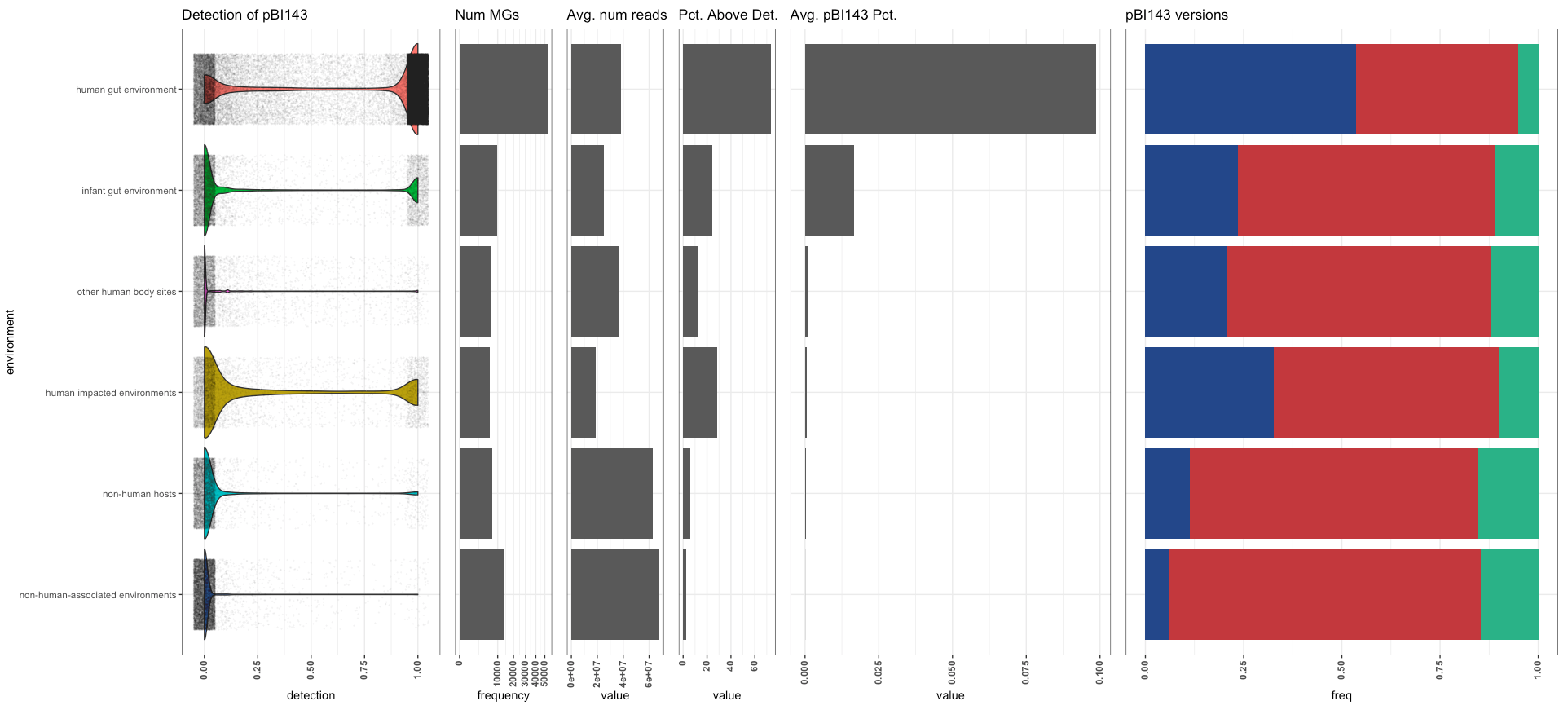
Read recruitment results summarized per ‘environment’ (raw output from R)
And we polished it in Inkscape as our main figure:
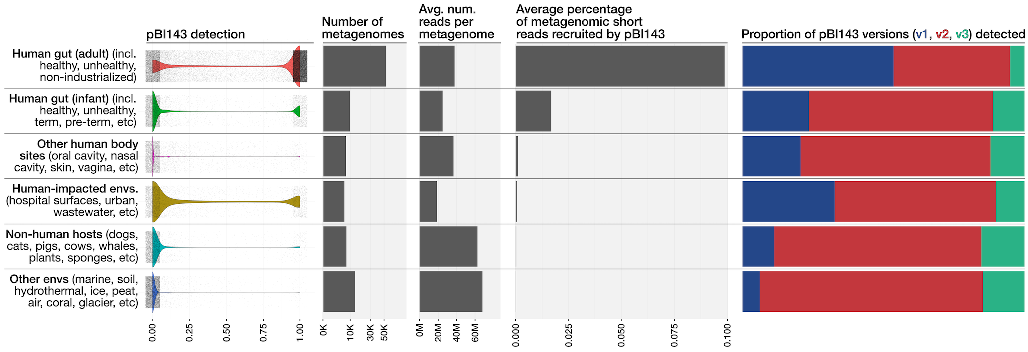
Read recruitment results summarized per ‘environment’ (after polishing in Inkscape)
We then generated a more comprehensive visualization of the 100K metagenomes for each biome,
human_gut_environment <- GET_ORDERED_AVERAGES(df[df$biome %in% human_gut_environment, ], 'biome', 'percent_reads_recruited')$name
infant_gut_environment <- GET_ORDERED_AVERAGES(df[df$biome %in% infant_gut_environment, ], 'biome', 'percent_reads_recruited')$name
non_gut_human_environments <- GET_ORDERED_AVERAGES(df[df$biome %in% non_gut_human_environments, ], 'biome', 'percent_reads_recruited')$name
human_impacted_environments_order <- GET_ORDERED_AVERAGES(df[df$biome %in% human_impacted_environments, ], 'biome', 'percent_reads_recruited')$name
non_human_associated_environments_order <- GET_ORDERED_AVERAGES(df[df$biome %in% non_human_associated_environments, ], 'biome', 'percent_reads_recruited')$name
non_human_hosts_order <- GET_ORDERED_AVERAGES(df[df$biome %in% non_human_hosts, ], 'biome', 'percent_reads_recruited')$name

biomes_order <- mergeLists(list(non_human_associated_environments_order),
                           list(human_impacted_environments_order),
                           list(non_human_hosts_order),
                           list(non_gut_human_environments),
                           list(infant_gut_environment),
                           list(human_gut_environment))[[1]]

PLOT_DF(df, biomes_order)
The polishing of the output image looked like this,
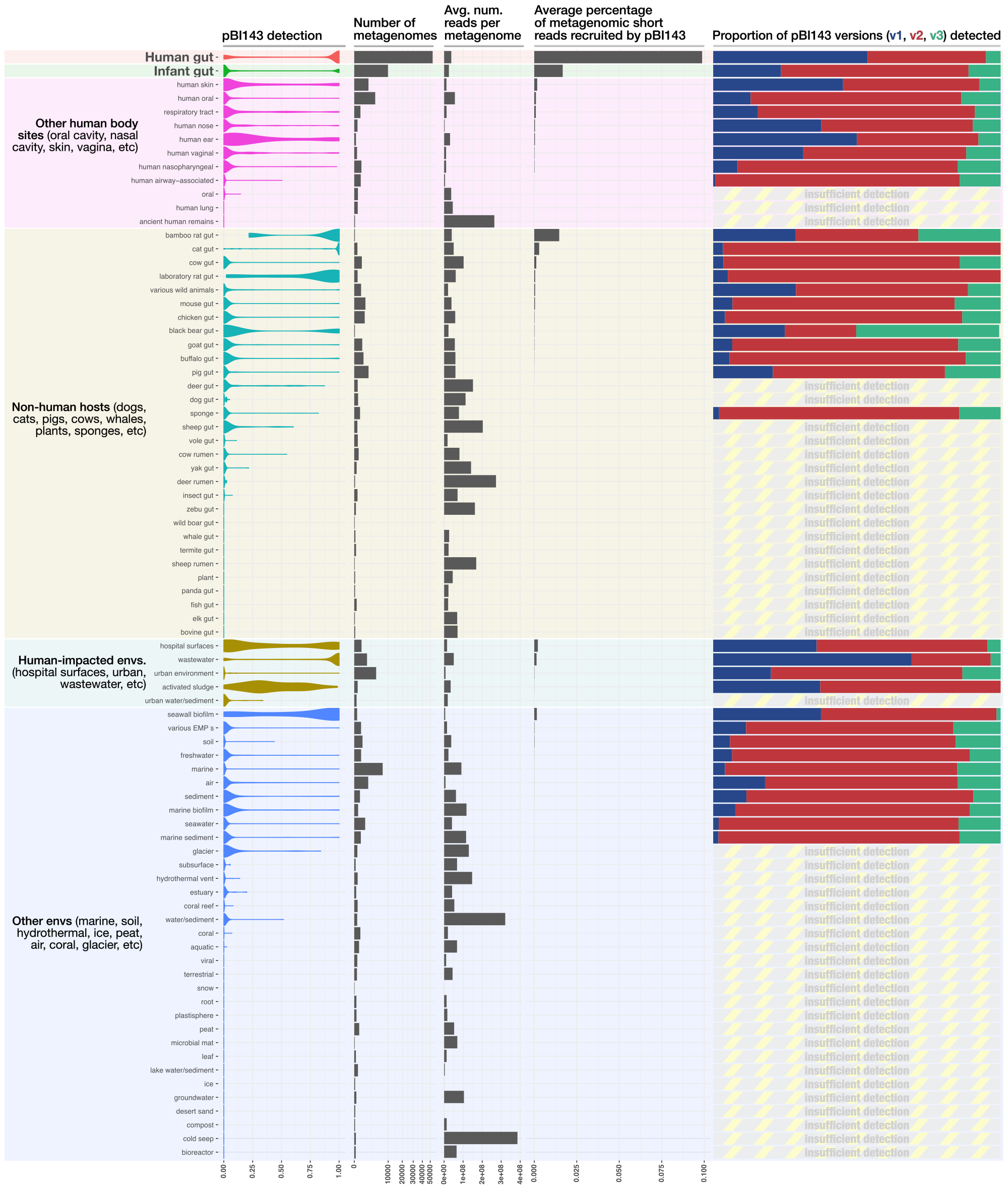
Read recruitment results per biome (after polishing in Inkscape)
Additional insights into read recruitment results
Overall, pBI143 was indeed absent in all non-host environmental samples, save those impacted by humans. For example, in open ocean samples, pBI143 is virtually absent (0.0000021% of reads on average, ~0.05X coverage), but in metagenomes collected close to a seawall pBI143 is convincingly present (0.002% of reads on average, ~7.3X coverage). Given the high presence of pBI143 in sewage, the seawall metagenomes almost certainly contain sewage and other wastewater. pBI143 is also convincingly present on hospital surfaces, another environment likely to contain trace amounts of human feces (0.002% of reads on average, ~8.7X coverage).
In addition to humans, this analysis comprehensively addressed whether pBI143 was present in other animals using gut metagenomes from buffalo, cat, chicken, cow, deer, dog, elk, fish, goat, insect, macaques, mouse, panda, pig, rat, sheep, termite, vole, whale, boar, yak, and zebu. Aside from humans, all meaningful signal was absent from other animals except cats and rats. Datasets surveyed here include metagenomes from human skin and oral cavity, which enabled us to understand if pBI143 was present in human microbiomes besides the gut microbiome. Unlike the extremely high presence of pBI143 in the human gut (0.1% of reads on average, ~1600X coverage), pBI143 was poorly detected both in samples from skin (0.002% of reads on average, ~4.6X coverage) and the oral cavity (0.0000003% of reads on average, ~0.006X coverage), which overall highlights the human gut-specific nature of pBI143.
So, what about the curious case of pBI143 in cats and rats? The absence of any meaningful signal for pBI143 from all host-associated gut environments except cats and rats sounds intriguing, but it is important to keep in mind that the coverage signal for pBI143 in these animals were 2 orders of magnitude less than in humans, and we found the non-spurious detection of pBI143 across all of the animals in these cohorts suspicious. We do not have a clear answer to the question why a plasmid that is completely absent in dogs, primates, pigs, or mice would be in cats and rats. One reasonable hypothesis to explain this anomaly could be that the presence of pBI143 in the cat and rat cohorts is due to contamination associated with sample preparation. The contamination hypothesis can further explain occasional occurrences of pBI143 in only one of many samples in a single animal species or its occasional occurrence in only one of many samples from marine or lake systems. But this hypothesis poorly applies to the case of cats, since unlike any other animal species tested, our qPCR assay did amplify trace levels of pBI143 from cat samples. So it is a high possibility that pBI143 is indeed present at extremely low abundances in cats. We further investigated cat and rat metagenomes and asked whether we observe the same level of genetic heterogeneity of pBI143 we observe in humans. Interestingly, upon a closer inspection of the individual coverage plots of pBI143 and single nucleotide variants, we found that virtually every sample within our cohort of 88 cats had identical SNVs and coverage plots. The same was true in rats:
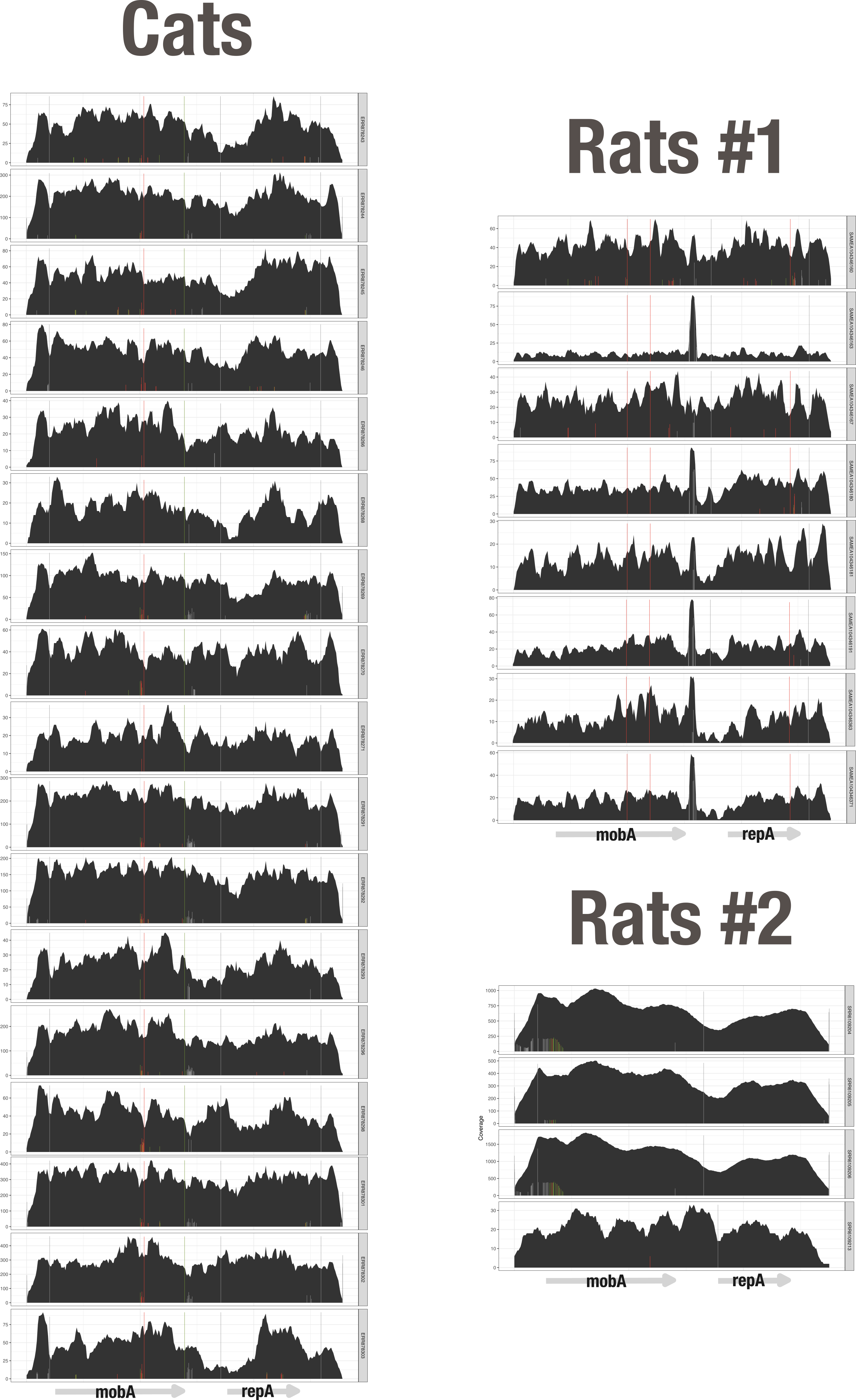
Coverage plots for pBI143-positive cat and rat cohorts
The complete lack of variation in pBI143 sequences and sequence coverage patterns in cat and rat metagenomes is extremely unexpected and suggests that it is unlikely that pBI143 is a naturally occurring member of cat gut metagenomes. While all these data suggest that low levels of a single version pBI143 may have been accidentally introduced to samples during the extraction or sequencing process, the faint yet positive qPCR signal from a different cohort of cats indicate that the route by which pBI143 ends up in cats may be much more complicated than contamination from humans during sample preparation.
Analyzing mother-infant metagenomes to find evidence for plasmid transfer through single-nucleotide variants (SNVs)
The purpose of the following workflow is to use read recruitment results obtained from multiple mother-infant gut metagenomes using pBI143 Version 1 sequence to investigate whether unique SNVs occur primarily between family members.
If you are planning to reproduce this workflow, I would suggest you to download this jupyter notebook file on your computer, and follow it from within your local jupyter environment. If you wish to do that, all you need to do is the following, assuming you are in an anvio-dev installed environment (the installation instructions for anvio-dev is here):
- Download this file on your computer.
- In your terminal go to the directory in which you have downloaded the file.
- In your terminal type
jupyter notebook, and selectpBI143_SNVs.ipynbto start.
Alternatively, you can read through the following steps and look at the output files the workflow reports.
Acquiring the data pack
The primary input for this analysis is anvi’o project files for four mother-infant datasets from Finland, Italy, Sweden, and the United States. The generation of these project files is very straightforward with the program anvi-run-workflow, to which we essentially provided the plasmid sequence and a list of metagenomes of interest. The program anvi-run-workflow simply (1) recruited reads using the plasmid sequence from each metagenome it was given, (2) profiled each read recruitment result using the program anvi-profile, and finally (3) merged all single profile databases using the program anvi-merge. We then moved these final anvi’o project files into four directories (which we will download for reproducibility in a second), where each directory contained a single contigs-db and a single merged profile-db that will enable us to perform the analyses down below.
Let’s start with downloading the data pack, which is at doi:10.6084/m9.figshare.22298215. In this jupyter notebook environment, I will use an anvi’o function to directly download it to my work directory:
# from anvi'o utils library import necessary functions
from anvio.utils import download_file, gzip_decompress_file, tar_extract_file

# instruct jupyter notebook to download the datapack
download_file('https://api.figshare.com/v2/file/download/39659905',
              output_file_path='MOTHER_INFANT_pBI143_POP_GEN.tar.gz')

# if we are here, the download is finished. now we will
# first decompress it (and get rid of the original file
# while at it).
gzip_decompress_file('MOTHER_INFANT_pBI143_POP_GEN.tar.gz',
                     keep_original=False)

# and finally untar it so we have a clean directory:
tar_extract_file('MOTHER_INFANT_pBI143_POP_GEN.tar',
                 output_file_path='.',
                 keep_original=False)
Running the lines above must have created a new directory called MOTHER_INFANT_pBI143_POP_GEN in our work directory. Run the ls command to confirm:
ls
MOTHER_INFANT_pBI143_POP_GEN/
Where the data pack directory should contain four folders as promised:
ls MOTHER_INFANT_pBI143_POP_GEN
README.txt fin/ ita/ swe/ usa/
With anvi’o contigs-db and profile-db files in them:
ls MOTHER_INFANT_pBI143_POP_GEN/*/
MOTHER_INFANT_pBI143_POP_GEN/fin/:

AUXILIARY-DATA.db  CONTIGS.db  PROFILE.db


MOTHER_INFANT_pBI143_POP_GEN/ita/:

AUXILIARY-DATA.db  CONTIGS.db  PROFILE.db


MOTHER_INFANT_pBI143_POP_GEN/swe/:

AUXILIARY-DATA.db  CONTIGS.db  PROFILE.db


MOTHER_INFANT_pBI143_POP_GEN/usa/:

AUXILIARY-DATA.db  CONTIGS.db  PROFILE.db
Good. Now we have the raw recruitment results described as anvi’o project files. Now we will change our work directory to the root of the data pack, and start playing with these data:
import os
os.chdir('MOTHER_INFANT_pBI143_POP_GEN')
Analysis
Unlike the vast majority of data analyses we do with anvi’o using anvi’o programs, here we will perform this analysis by accessing anvi’o libraries directly from within Python scripts we will implement below. Many of these steps use anvi’o functionality that is accessible through two anvi’o programs:
- anvi-gen-variability-profile (which is a program that gives us access to nucleotide, codon, or amino acid variants in metagenomic read recruitment results),
- anvi-gen-variability-network (which is a program that turns an anvi’o nucleotide variability report into a Gephi compatible XML network file).
But by accessing anvi’o libraries directly, we get to apply filtering rules that are dependent on sample names, such as removing infants from the dataset whose mother does not have a metagenome and vice versa. One could indeed implement those steps after getting the necessary output files from anvi-gen-variability-profile using R, EXCEL or by manually selecting samples to be considered for the analysis. But a Pythonic approach helps with reproducibility, and reduces human error.
The actual bottom line is the following: these analyses can be done with anvi’o without writing a single line of Python code, too. In addition to reproducibility, a side purpose of this workflow is to show those who might be interested in exploring anvi’o deeper what else can be done with it. So here we are.
Our analysis starts with importing some libraries that will be necessary later (of course, at the beginning of the analysis we didn’t know which libraries were necessary, but we expanded this section as we made progress with the code):
import argparse
import pandas as pd

import anvio.terminal as terminal
import anvio.filesnpaths as filesnpaths

from anvio.variabilityops import NucleotidesEngine
from anvio.utils import store_dataframe_as_TAB_delimited_file

run = terminal.Run(width=27)
Here we define a Python function that takes a set of anvi’o proifle-db and contigs-db files, and returns a comprehensive dictionary for the nucleotide variation per position:
def get_snvs(contigs_db_path, profile_db_path):
    args = argparse.Namespace(contigs_db=contigs_db_path,
                              profile_db=profile_db_path,
                              gene_caller_ids='0',
                              compute_gene_coverage_stats=True)

    n = NucleotidesEngine(args, r=terminal.Run(verbose=False), p=terminal.Progress(verbose=False))
    n.process()

    return n.data
Please note that this is done by passing a set of arguments to the NucleotidesEngine class that we imported from anvio.variabilityops. We learned what to import from ths library and how to format the args from the source code of anvi-gen-variability-profile program. Please also note the gene_caller_ids=0 directive among the arguments passed to the class. The gene caller id 0 corresponds to the mobA gene in pBI143. Since our intention was to focus on mobA, here we limit all data we will acquire from the NucleotidesEngine class to that gene.
The next function is a more complex one, but its sole purpose is to work with the sample names (which include information such as the unique family identifier, or whether a given sample belongs to the mother or an infant, etc) to summarize information about the mother-infant pairs remaining in our dataset, which is passed to the function as udf:
def mother_infant_pair_summary(udf, drop_incomplete_families=False):
    # learn all the sample names that are present in the dataframe
    sample_names = list(udf.sample_id.unique())

    def get_countries(family_names):
        # learn which countries are present in the datsaet by
        # splitting that piece of information from sample names
        country_names = [s.split('_')[0] for s in family_names]
        return dict(zip(list(country_names), [country_names.count(i) for i in country_names]))

    # we will create this intermediate dictionary to resolve sample names into
    # some meaningful information about mother-infant pairs
    mother_infant_pairs = {}
    for sample_name in sample_names:
        family_name = '_'.join(sample_name.split('_')[0:2])[:-1]
        participant = sample_name.split('_')[1][-1]
        day = sample_name.split('_')[2]

        if family_name not in mother_infant_pairs:
            mother_infant_pairs[family_name] = {'M': [], 'C': []}

        mother_infant_pairs[family_name][participant].append(day)

    # now we can learn about family names that include at least one mother
    # and one infant:
    family_names_with_both_M_and_C = [p for p in mother_infant_pairs if mother_infant_pairs[p]['M'] and mother_infant_pairs[p]['C']]

    # now we subset the broader dictionary to have one that only includes
    # complete families (this is largely for reporting purposes)
    mother_infant_pairs_with_both_mother_and_infant = {}
    for family_name in family_names_with_both_M_and_C:
        mother_infant_pairs_with_both_mother_and_infant[family_name] = mother_infant_pairs[family_name]

    # report some reports .. these will be printed to the user's screen
    # when this function is called
    run.info('Num entires', f"{len(udf.index)}")
    run.info('Num samples', f"{udf.sample_id.nunique()}")
    run.info('Num families', f"{len(mother_infant_pairs)} / {get_countries(mother_infant_pairs.keys())}")
    run.info('   w/both members', f"{len(mother_infant_pairs_with_both_mother_and_infant)} / {get_countries(mother_infant_pairs_with_both_mother_and_infant.keys())}")

    if drop_incomplete_families:
        # reconstruct the original sample names for complete families:
        sample_names_for_families_with_both_M_and_C = []
        for family_name in mother_infant_pairs_with_both_mother_and_infant:
            for day in mother_infant_pairs_with_both_mother_and_infant[family_name]['M']:
                sample_names_for_families_with_both_M_and_C.append(f"{family_name}M_{day}")
            for day in mother_infant_pairs_with_both_mother_and_infant[family_name]['C']:
                sample_names_for_families_with_both_M_and_C.append(f"{family_name}C_{day}")

        # return a new dataframe after dropping all sample names from incomplete families
        # so we have a dataframe that is clean and reprsent only complete families (sad)
        return udf[udf['sample_id'].isin(sample_names_for_families_with_both_M_and_C)]
    else:
        pass
Now it is time to get single-nucleotide variant data for the mother-infant pairs from Finland, Sweden, USA, and Italy using the anvi’o project files we downloaded using the data pack before, using the fancy function get_snvs we defined above.
It is important to note that the resulting data frames will contain information only for samples that include at least one SNV in the mobA gene of the plasmid. This means, samples that have no SNVs will not be reported in the following data frames even though they were in the original dataset.
df_fin = get_snvs('fin/CONTIGS.db', 'fin/PROFILE.db')

df_swe = get_snvs('swe/CONTIGS.db', 'swe/PROFILE.db')

df_usa = get_snvs('usa/CONTIGS.db', 'usa/PROFILE.db')

df_ita = get_snvs('ita/CONTIGS.db', 'ita/PROFILE.db')

# combine all data frames
df = pd.concat([df_fin, df_swe, df_usa, df_ita])

# reset the `entry_id` column to make sure each entry has a
# unique identifier:
df['entry_id'] = range(0, len(df))
Now we take a quick look at the resulting data frame that combines all data from all samples by simply sending this data frame to the function mother_infant_pair_summary implemented above, so you can appreciate its true utility:
mother_infant_pair_summary(df)
Num entires ................: 8183
Num samples ................: 309
Num families ...............: 102 / {'FIN': 15, 'SWE': 52, 'USA': 24, 'ITA': 11}
   w/both members ..........: 57 / {'FIN': 3, 'SWE': 36, 'USA': 16, 'ITA': 2}
The data frame df is quite a comprehensive one, as anvi’o generates an extremely rich output file to describe variants observed in metagenomes. We can take a very quick look, and go through the columns to have an idea (they scroll right):
df
| entry_id | sample_id | split_name | pos | pos_in_contig | corresponding_gene_call | in_noncoding_gene_call | in_coding_gene_call | base_pos_in_codon | codon_order_in_gene | coverage | cov_outlier_in_split | cov_outlier_in_contig | departure_from_reference | competing_nts | reference | A | C | G | T | N | codon_number | unique_pos_identifier_str | gene_length | unique_pos_identifier | contig_name | consensus | departure_from_consensus | n2n1ratio | entropy | gene_coverage | non_outlier_gene_coverage | non_outlier_gene_coverage_std | mean_normalized_coverage |
|---|---|---|---|---|---|---|---|---|---|---|---|---|---|---|---|---|---|---|---|---|---|---|---|---|---|---|---|---|---|---|---|---|---|
| 0 | FIN_0018M_000A | pBI143_V1 | 569 | 569 | 0 | 0 | 1 | 3 | 89 | 60 | 0 | 0 | 1.000000 | TT | C | 0 | 0 | 0 | 60 | 0 | 90 | pBI143_V1 | 1104 | 0 | pBI143_V1 | T | 0.000000 | 0.000000 | 0.000000 | 54.063406 | 52.346307 | 6.167071 | 1.109808 |
| 1 | FIN_0072M_000A | pBI143_V1 | 344 | 344 | 0 | 0 | 1 | 3 | 14 | 115 | 0 | 0 | 0.947826 | CT | T | 0 | 109 | 0 | 6 | 0 | 15 | pBI143_V1 | 1104 | 1 | pBI143_V1 | C | 0.052174 | 0.055046 | 0.204867 | 131.563406 | 127.259220 | 16.885726 | 0.874103 |
| 2 | FIN_0072M_000A | pBI143_V1 | 389 | 389 | 0 | 0 | 1 | 3 | 29 | 135 | 0 | 0 | 0.955556 | CG | C | 0 | 6 | 129 | 0 | 0 | 30 | pBI143_V1 | 1104 | 2 | pBI143_V1 | G | 0.044444 | 0.046512 | 0.181820 | 131.563406 | 127.259220 | 16.885726 | 1.026121 |
| 3 | FIN_0072M_000A | pBI143_V1 | 446 | 446 | 0 | 0 | 1 | 3 | 48 | 137 | 0 | 0 | 0.970803 | AG | A | 4 | 0 | 133 | 0 | 0 | 49 | pBI143_V1 | 1104 | 3 | pBI143_V1 | G | 0.029197 | 0.030075 | 0.131940 | 131.563406 | 127.259220 | 16.885726 | 1.041323 |
| 4 | FIN_0072M_000A | pBI143_V1 | 458 | 458 | 0 | 0 | 1 | 3 | 52 | 114 | 0 | 0 | 0.956140 | AG | A | 5 | 0 | 109 | 0 | 0 | 53 | pBI143_V1 | 1104 | 4 | pBI143_V1 | G | 0.043860 | 0.045872 | 0.180022 | 131.563406 | 127.259220 | 16.885726 | 0.866502 |
| ... | ... | ... | ... | ... | ... | ... | ... | ... | ... | ... | ... | ... | ... | ... | ... | ... | ... | ... | ... | ... | ... | ... | ... | ... | ... | ... | ... | ... | ... | ... | ... | ... | ... |
| 8178 | ITA_006C_001D | pBI143_V1 | 1400 | 1400 | 0 | 0 | 1 | 3 | 366 | 25 | 1 | 1 | 0.960000 | AG | G | 24 | 0 | 1 | 0 | 0 | 367 | pBI143_V1 | 1104 | 89 | pBI143_V1 | A | 0.040000 | 0.041667 | 0.167944 | 134.579710 | 134.309496 | 29.018131 | 0.185764 |
| 8179 | ITA_024M_000D | pBI143_V1 | 782 | 782 | 0 | 0 | 1 | 3 | 160 | 21 | 0 | 0 | 0.238095 | CT | C | 0 | 16 | 0 | 5 | 0 | 161 | pBI143_V1 | 1104 | 29 | pBI143_V1 | C | 0.238095 | 0.312500 | 0.548874 | 13.516304 | 13.027230 | 5.382654 | 1.553679 |
| 8180 | ITA_024M_000D | pBI143_V1 | 860 | 860 | 0 | 0 | 1 | 3 | 186 | 27 | 1 | 1 | 0.185185 | AC | A | 22 | 5 | 0 | 0 | 0 | 187 | pBI143_V1 | 1104 | 34 | pBI143_V1 | A | 0.185185 | 0.227273 | 0.479166 | 13.516304 | 13.027230 | 5.382654 | 1.997587 |
| 8181 | ITA_024M_000D | pBI143_V1 | 1050 | 1050 | 0 | 0 | 1 | 1 | 250 | 15 | 0 | 0 | 0.266667 | AG | G | 4 | 0 | 11 | 0 | 0 | 251 | pBI143_V1 | 1104 | 47 | pBI143_V1 | G | 0.266667 | 0.363636 | 0.579915 | 13.516304 | 13.027230 | 5.382654 | 1.109771 |
| 8182 | ITA_017C_003D | pBI143_V1 | 654 | 654 | 0 | 0 | 1 | 1 | 118 | 67 | 1 | 1 | 0.089552 | AG | A | 61 | 0 | 6 | 0 | 0 | 119 | pBI143_V1 | 1104 | 90 | pBI143_V1 | A | 0.089552 | 0.098361 | 0.301501 | 52.745471 | 50.215139 | 10.296381 | 1.270251 |
8183 rows × 34 columns
While this is our raw data frame that contains all variants from all samples that had at least one variable nucleotide position in the mobA gene, it needs some cleaning.
For instance, in some samples the mobA gene will have a pretty low coverage to perform a robust analysis of SNV patterns, and such samples should be removed first. Here are some of the samples that have the lowest coverage values:
sorted(df.gene_coverage.unique())[:20]
[3.2454710144927534,
 4.181159420289855,
 4.6231884057971016,
 4.684782608695652,
 5.2853260869565215,
 6.155797101449275,
 6.183876811594203,
 6.631340579710145,
 6.665760869565218,
 6.7644927536231885,
 7.306159420289855,
 7.406702898550725,
 7.54981884057971,
 7.729166666666667,
 7.913949275362318,
 8.008152173913043,
 8.177536231884059,
 9.181159420289855,
 10.353260869565217,
 10.72463768115942]
For a very stringent analysis, here we can drop samples from our data frame where the mobA gene has less than 50X coverage:
dfx = df.drop(df[df.gene_coverage < 50].index)
The new data frame dfx only contains samples that have enough reads to cover mobA at 50X or more. But as you can imagine, this removal step does not include any logic to ‘maintain’ families in the dataset. Following the removal of samples based on the coverage of mobA, now there will be some infants without mother samples, and some mother samples with no infants. Since the purpose of this analysis to investigate plasmid transfer through SNVs, we don’t need those samples.
And mother_infant_pair_summary comes to our rescue once again, as we request this function to further drop samples from dfx that belong to ‘incomplete’ families:
dfx = mother_infant_pair_summary(dfx, drop_incomplete_families=True)
Num entires ................: 6076
Num samples ................: 245
Num families ...............: 87 / {'FIN': 12, 'SWE': 48, 'USA': 21, 'ITA': 6}
   w/both members ..........: 49 / {'FIN': 2, 'SWE': 33, 'USA': 13, 'ITA': 1}
In our final dataset, we have 49 families for which at least one mother metagenome and one infant metagenome was present.
At this point we can report this final data frame as a TAB-delimited file, an output that will be identical to an output anvi-gen-variability-profile would have generated:
# this is the file name in which we will store all the
# final varaibility data:
variability_profile_path = "pBI143_SNVs.txt"

dfx.reset_index(drop=True, inplace=True)
dfx["entry_id"] = dfx.index

# order by [corresponding_gene_call, codon_order_in_gene]
dfx = dfx.sort_values(by = ["corresponding_gene_call", "codon_order_in_gene"])

# ask anvi'o to store it:
store_dataframe_as_TAB_delimited_file(dfx,
                                      variability_profile_path,
                                      columns=dfx.columns.tolist())
'pBI143_SNVs.txt'
If you wish, you can take a look at it in your terminal.
The next step is to represent the information in this file as a network so we can visualize the relationships between all samples in the dataset with respect to their shared SNVs using Gephi. But first, we would like to generate a dictionary with sample information using sample names, so we can highlight samples that belong to the same family, etc.
For this, we will parse the sample names, and create a dictionary, sample_information_dict, to pass to the VariabiltyNetwork class below:
# an empty dictionary
sample_information_dict = {}

# get the final sample names from `dfx`
sample_names = list(dfx.sample_id.unique())

# go through each sample name, split it into pieces,
# based on the `_` character, and fill in the
# dictionary
for sample_name in sample_names:
    family_name = '_'.join(sample_name.split('_')[0:2])[:-1]
    participant = sample_name.split('_')[1][-1]
    day = sample_name.split('_')[2]
    country = family_name.split('_')[0]

    sample_information_dict[sample_name] = {'family_name': family_name,
                                            'participant': participant,
                                            'country': country,
                                            'sample_name': sample_name,
                                            'coverage': dfx[dfx.sample_id == sample_name].gene_coverage.tolist()[0]}
The resulting is a very simple data structure that looks like this:
sample_information_dict
    {'SWE_0100C_360D': {'family_name': 'SWE_0100',
                        'participant': 'C',
                        'country': 'SWE',
                        'sample_name': 'SWE_0100C_360D',
                        'coverage': 209.56159420289856},
     'FIN_0226C_014D': {'family_name': 'FIN_0226',
                        'participant': 'C',
                        'country': 'FIN',
                        'sample_name': 'FIN_0226C_014D',
                        'coverage': 103.84510869565217},
     'FIN_0226C_030D': {'family_name': 'FIN_0226',
                        'participant': 'C',
                        'country': 'FIN',
                        'sample_name': 'FIN_0226C_030D',
                        'coverage': 101.2038043478261},
     'FIN_0226C_090D': {'family_name': 'FIN_0226',
                        'participant': 'C',
                        'country': 'FIN',
                        'sample_name': 'FIN_0226C_090D',
                        'coverage': 58.583333333333336},
     'FIN_0226M_000A': {'family_name': 'FIN_0226',
                        'participant': 'M',
                        'country': 'FIN',
                        'sample_name': 'FIN_0226M_000A',
                        'coverage': 250.69927536231884},
     'FIN_0226M_000B': {'family_name': 'FIN_0226',
                        'participant': 'M',
                        'country': 'FIN',
                        'sample_name': 'FIN_0226M_000B',
                        'coverage': 444.6847826086956},
     'FIN_0226M_090D': {'family_name': 'FIN_0226',
                        'participant': 'M',
                        'country': 'FIN',
                        'sample_name': 'FIN_0226M_090D',
                        'coverage': 551.0742753623189},
     'SWE_0005C_000D': {'family_name': 'SWE_0005',
                        'participant': 'C',
                        'country': 'SWE',
                        'sample_name': 'SWE_0005C_000D',
                        'coverage': 6812.400362318841},
     'SWE_0005C_120D': {'family_name': 'SWE_0005',
                        'participant': 'C',
                        'country': 'SWE',
                        'sample_name': 'SWE_0005C_120D',
                        'coverage': 2413.664855072464},
     'SWE_0005M_000D': {'family_name': 'SWE_0005',
                        'participant': 'M',
                        'country': 'SWE',
                        'sample_name': 'SWE_0005M_000D',
                        'coverage': 315.9284420289855},
     'SWE_0007C_360D': {'family_name': 'SWE_0007',
                        'participant': 'C',
                        'country': 'SWE',
                        'sample_name': 'SWE_0007C_360D',
                        'coverage': 2025.1358695652175},
     'SWE_0007M_000D': {'family_name': 'SWE_0007',
                        'participant': 'M',
                        'country': 'SWE',
                        'sample_name': 'SWE_0007M_000D',
                        'coverage': 552.3215579710145},
     'SWE_0008C_000D': {'family_name': 'SWE_0008',
                        'participant': 'C',
                        'country': 'SWE',
                        'sample_name': 'SWE_0008C_000D',
                        'coverage': 4070.4184782608695},
     'SWE_0008C_120D': {'family_name': 'SWE_0008',
                        'participant': 'C',
                        'country': 'SWE',
                        'sample_name': 'SWE_0008C_120D',
                        'coverage': 3511.5190217391305},
     'SWE_0008C_360D': {'family_name': 'SWE_0008',
                        'participant': 'C',
                        'country': 'SWE',
                        'sample_name': 'SWE_0008C_360D',
                        'coverage': 3447.538043478261},
     'SWE_0008M_000D': {'family_name': 'SWE_0008',
                        'participant': 'M',
                        'country': 'SWE',
                        'sample_name': 'SWE_0008M_000D',
                        'coverage': 256.16847826086956},
     'SWE_0011C_120D': {'family_name': 'SWE_0011',
                        'participant': 'C',
                        'country': 'SWE',
                        'sample_name': 'SWE_0011C_120D',
                        'coverage': 7212.425724637681},
      (...)
}
Now it is time to ask anvi’o to convert all this into an XML file:
from anvio.variabilityops import VariabilityNetwork

variability_network_path = "pBI143_SNVs.gexf"

args = argparse.Namespace(input_file=variability_profile_path,
                          include_competing_NTs='noise-robust',
                          output_file=variability_network_path)

variability_network = VariabilityNetwork(args, r=terminal.Run(verbose=False), p=terminal.Progress(verbose=False))
variability_network.samples_information_dict = sample_information_dict
variability_network.generate()
You can now open the resulting XML file, pBI143_SNVs.gexf, in Gephi to visualize this network. And that’s exactly what we did. We opened the file pBI143_SNVs.gexf in Gephi:
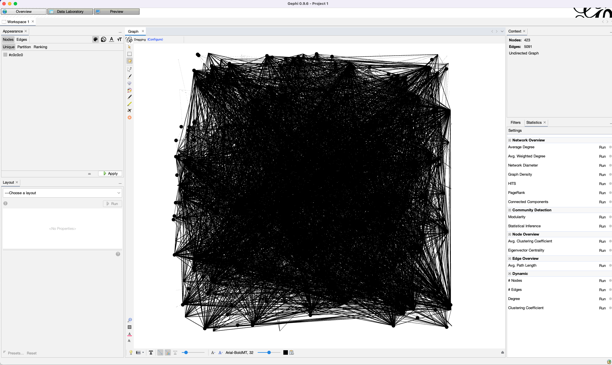
Upon opening the GEXF file of mother-infant variants in Gephi
Then we run the ForceAtlas2 algorithm with the options to dissuade hubs and LinLog mode with non-overlapping nodes while partitioning all nodes into ‘family’ bins (a piece of information that was available to Gephi thanks to the sample_information_dict we passed to the class VariabiltyNetwork) so we can see which samples belong to the same family:
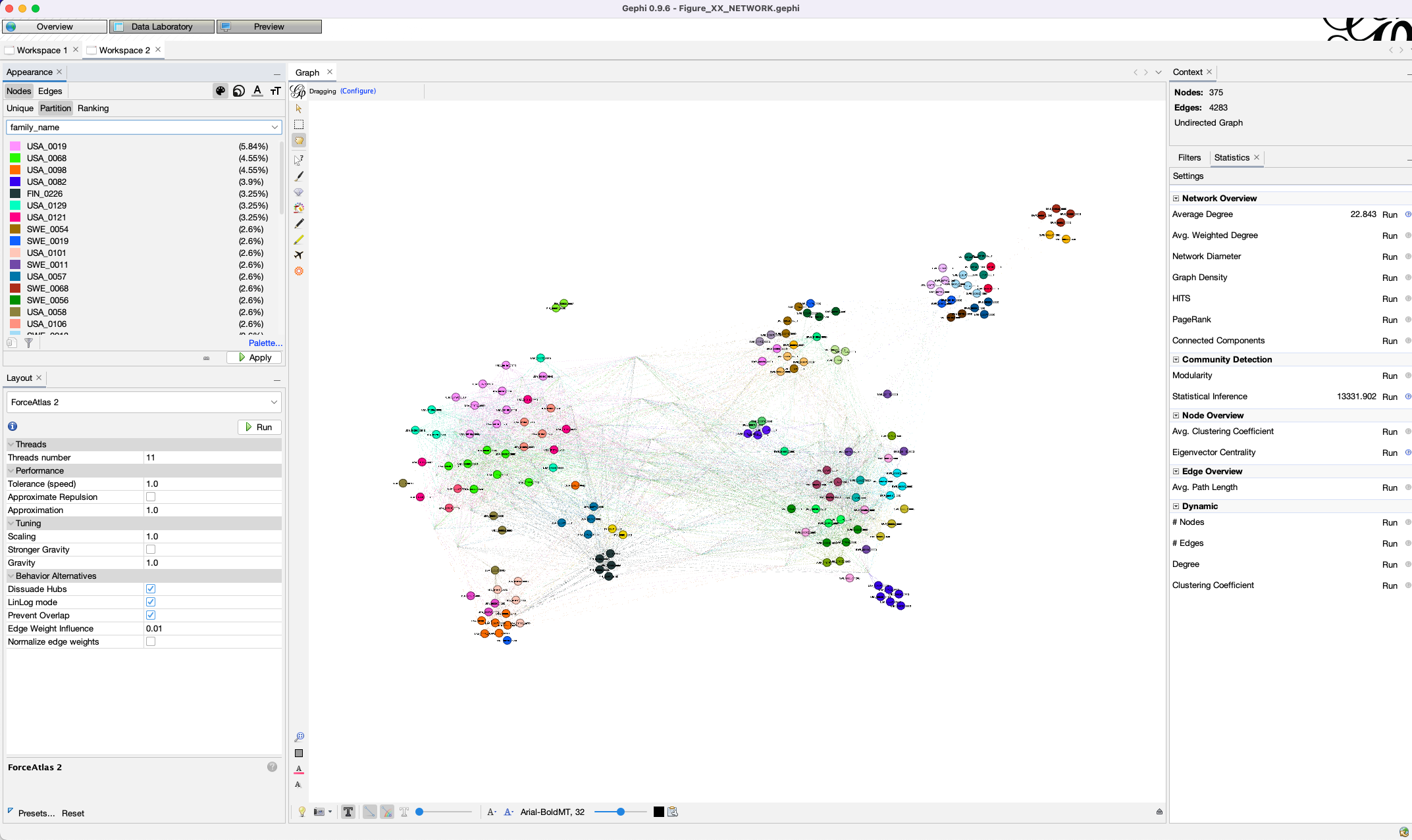
Following the convergence of ForceAtlas2 with some minor adjustments
We then switched to the Preview panel to export an SVG,
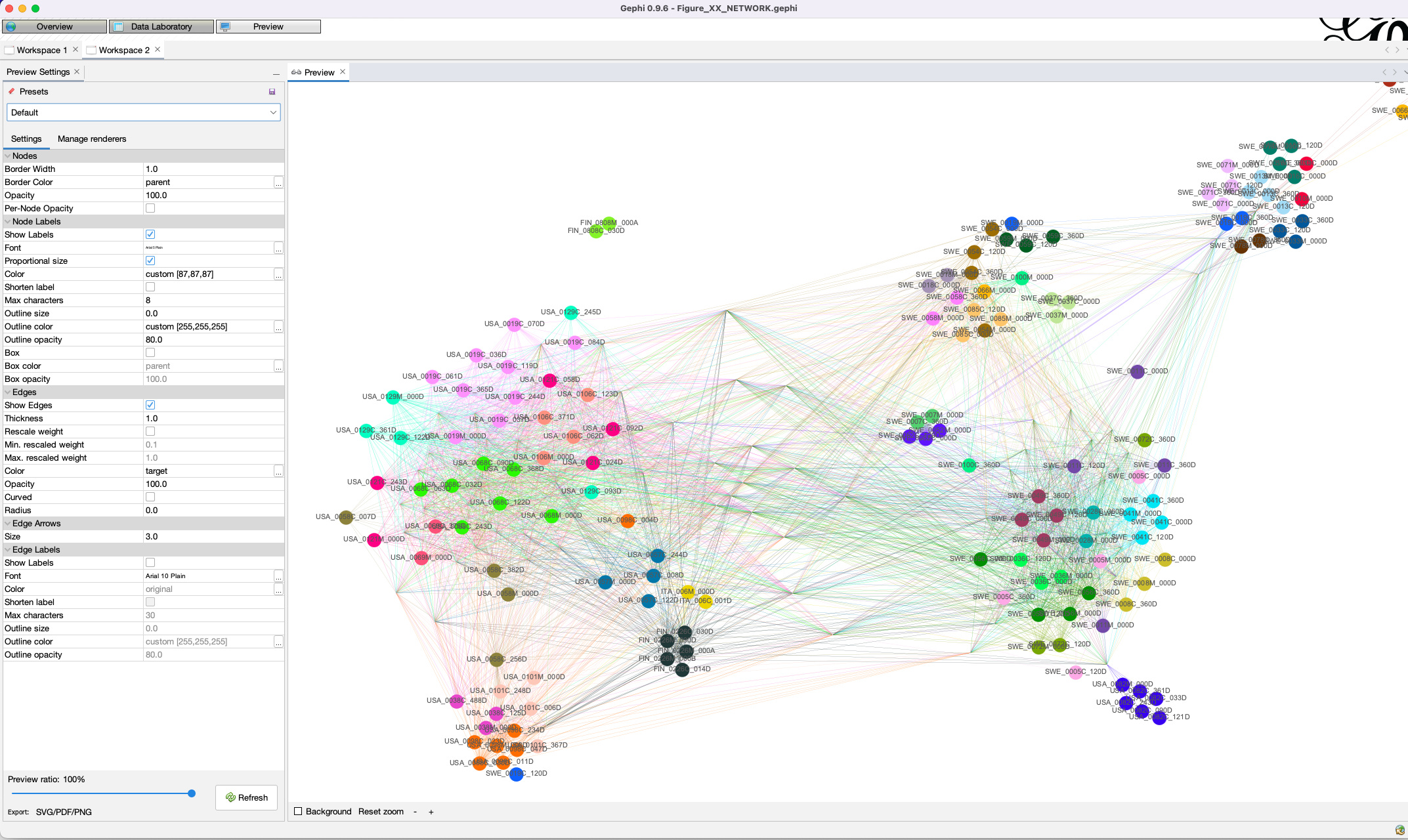
Jumping to the Preview panel to get an SVG with desired visual qualities (such as keeping the sample names big on the figure so we can later identify which sample was the mother sample for a given family, etc)
And we finalized this image for publication using Inkscape.