Single amino acid variants in SAR11
Table of Contents
- Single-amino acid variants reveal evolutionary processes that shape the biogeography of a global SAR11 subclade.
- Downloading the 21 SAR11 cultivar genomes
- Downloading the TARA Oceans and Ocean Sampling Day metagenomes
- Defining metagenomic sets, setting sample names, and linking those with the raw data
- Quality-filtering of raw reads
- Generating an anvi’o CONTIGS database
- Estimating distances between isolate genomes based on full-length 16S ribosomal RNA gene sequences
- Inferring functions with COGs
- Recruitment of metagenomic reads
- Profiling the mapping results with anvi’o
- Generating a merged anvi’o profile
- Generating a genomic collection
- Summarizing the collection ‘Genomes’
- Computing the pangenome
- Linking the pangenome to the environment
- Finding core S-LLPA genes with PDB matches
- Protein structure prediction
- Structural mapping of SAAVs
- Generating an interactive output
- Setting the stage
- The approach
- Loading the dataset
- Pseudo parent-class generation
- Learning Latent Annotations
- The entire flow in Python
- Generating distance matrices from fixation index for SAAVs and SNVs data
- Identifying proteotypes from Deep Learning and Fixation Index Distances
This document describes the reproducible bioinformatics workflow for our study titled “The large scale biogeography of amino acid variants within a single SAR11 population is governed by natural selection”. Here you will find program names and exact parameters we used throughout every step of the analysis of SAR11 genomes and metagenomes from the TARA Oceans and Ocean Sampling Day projects, which relied predominantly on the open-source analysis platform anvi’o (Eren et al., 2015).
Single-amino acid variants reveal evolutionary processes that shape the biogeography of a global SAR11 subclade.

- A first attempt to link population genetics and the predicted protein structures to explore in silico the intersection beetween protein biochemistry and evolutionary processes acting on an environmental microbe.
- An application of metapangenomics to define subclades of SAR11 based on gene content and ecology.
- Reproducible bioinformatics workflow is here. Reviewer criticism and our responses are also available.
All anvi’o analyses in this document are performed using the anvi’o version v5. Please see the installation notes to download the appropriate version through PyPI, Docker, or GitHub.
The URL http://merenlab.org/data/sar11-saavs/ serves the most up-to-date version of this document.
Summary
In this study,
-
We characterized the metapangenome of 21 SAR11 isolate genomes (subclades)using metagenomes from the TARA Oceans and Ocean Sampling Day projects,
-
Identified a remarkably abundant and widespread SAR11 lineage with considerable yet cohesive levels of variation, as measured by the alignment quality of recruited reads.
-
Analysed single-nucleotide variants (SNVs) and single-amino acid variants (SAAVs), and linked SAAVs to predicted tertiary structures of core proteins
-
Estimated distances between metagenomes based on SAAVs using Deep Learning,
Sections in this document will detail all the steps of downloading and processing SAR11 genomes and metagenomes, mapping metagenomic reads onto the SAR11 genomes, identifying and processing genomic variability to explore the amino acid diversification traits of a finely resolved SAR11 lineage.
Please feel free to leave a comment, or send an e-mail to us if you have any questions.
Setting the stage
This section explains how to download a set of 21 SAR11 genomes and download and quality filter short metagenomic reads from the TARA Oceans project (Sunagawa et al., 2015) and Ocean Sampling Day project (Kopf et al., 2015).
The TARA Oceans metagenomes we analyzed are publicly available through the European Bioinformatics Institute (EBI) repository and NCBI under project IDs ERP001736 and PRJEB1787, respectively.
Downloading the 21 SAR11 cultivar genomes
You can get a copy of the FASTA file containing all 21 SAR11 cultivar genomes into your work directory using this command line:
curl -L -O http://merenlab.org/data/sar11-saavs/files/SAR11-isolates.fa.gz
gzip -d SAR11-isolates.fa.gz
Downloading the TARA Oceans and Ocean Sampling Day metagenomes
This file contains URLs for FTP access for each raw data file for 103 samples, and you can get a copy of it into your work directory,
curl -L -O http://merenlab.org/data/sar11-saavs/files/ftp-links-for-raw-data-files.txt
and download each of the raw sequencing data file from the EMBL servers this way:
for url in `cat ftp-links-for-raw-data-files.txt`
do
    curl -L -O $url
done
This may take quite a while.
Defining metagenomic sets, setting sample names, and linking those with the raw data
We defined 12 ‘metagenomic sets’ for geographically bound locations TARA Oceans samples originated from, consistent with our previous work flow to reconstruct ~1,000 population genomes. We defined an additional metagenomic set for the 10 Ocean Sampling Day metagenomes that cover high-latitudes of the north hemisphere.
We tailored our sample naming schema for convenience and reproducibility. This file contains the three-letter identifiers for each of the 13 metagenomic sets, which will become prefixes for each sample name for direct access to all samples from a given metagenomic set. This file will be referred to as sets.txt throughout the document, and you can get a copy of this file into your work directory:
curl -L -O http://merenlab.org/data/sar11-saavs/files/sets.txt
We used these three-letter prefixes to name each of the 103 samples, and to associate them with metagenomic sets with which they were affiliated. This file contains sample names, and explains which raw data files are associated with each sample. It will be referred to as samples.txt throughout the document, and you can get a copy of this file into your work directory:
curl -L -O http://merenlab.org/data/sar11-saavs/files/samples.txt
TARA samples file should look like this:
$ wc -l samples.txt
      103 samples.txt
$ head samples.txt
sample     r1                            r2
MED_18_05M ERR599140_1.gz,ERR598993_1.gz ERR599140_2.gz,ERR598993_2.gz
MED_23_05M ERR315858_1.gz,ERR315861_1.gz ERR315858_2.gz,ERR315861_2.gz
MED_25_05M ERR599043_1.gz,ERR598951_1.gz ERR599043_2.gz,ERR598951_2.gz
MED_30_05M ERR315862_1.gz,ERR315863_1.gz ERR315862_2.gz,ERR315863_2.gz
RED_31_05M ERR599106_1.gz,ERR598969_1.gz ERR599106_2.gz,ERR598969_2.gz
RED_32_05M ERR599041_1.gz,ERR599116_1.gz ERR599041_2.gz,ERR599116_2.gz
RED_33_05M ERR599049_1.gz,ERR599134_1.gz ERR599049_2.gz,ERR599134_2.gz
RED_34_05M ERR598959_1.gz,ERR598991_1.gz ERR598959_2.gz,ERR598991_2.gz
ION_36_05M ERR599143_1.gz,ERR598966_1.gz ERR599143_2.gz,ERR598966_2.gz
This file above also represents the standard input for illumina-utils library for processing the raw metagenomic data for each sample.
Quality-filtering of raw reads
We used the illumina-utils library v1.4.1 (Eren et al., 2013) to remove noise from raw reads prior to mapping.
To produce the configuration files illumina utils requires, we first run the program iu-gen-configs on the file samples.txt:
iu-gen-configs samples.txt
This step should generate 103 config files with the extension of .ini in the working directory.
To perform the quality filtering on samples config files describe, we used the program iu-filter-quality-minoche with default parameters, which implements the approach detailed in Minoche et al. (Minoche et al., 2011):
for sample in `awk '{print $1}' samples.txt`
do
    if [ "$sample" == "sample" ]; then continue; fi
    iu-filter-quality-minoche $sample.ini --ignore-deflines
done
This step generated files that summarize the quality filtering results for each sample. Here is an example for one:
$ cat ASW_82_40M-STATS.txt
number of pairs analyzed      : 222110286
total pairs passed            : 204045433 (%91.87 of all pairs)
total pairs failed            : 18064853 (%8.13 of all pairs)
  pairs failed due to pair_1  : 3237955 (%17.92 of all failed pairs)
  pairs failed due to pair_2  : 8714230 (%48.24 of all failed pairs)
  pairs failed due to both    : 6112668 (%33.84 of all failed pairs)
  FAILED_REASON_N             : 302725 (%1.68 of all failed pairs)
  FAILED_REASON_C33           : 17762128 (%98.32 of all failed pairs)
This step also generated FASTQ files for each sample that contain quality-filtered reads for downstream analyses. The resulting *-QUALITY_PASSED_R*.fastq.gz files in the work directory represent the main inputs for mapping.
Mapping metagenomic reads to SAR11 genomes
This section explains various steps to characterize the occurrence of each SAR11 isolate genome in metagenomes.
Generating an anvi’o CONTIGS database
We used the program anvi-gen-contigs-database with default parameters to profile all contigs for SAR11 isolate genomes, and generate an anvi’o contigs database that stores for each contig the DNA sequence, GC-content, tetranucleotide frequency, and open reading frames as Prodigal v2.6.3 (Hyatt et al., 2010) identifies them:
anvi-gen-contigs-database -f SAR11-isolates.fa \
                          -o SAR11-CONTIGS.db
The open reading frames identified by Prodigal can be exported with the following command:
anvi-export-gene-calls -c SAR11-CONTIGS.db \
                       -o gene_calls_summary.txt
doi:10.5281/zenodo.835218 serves the resulting contigs database.
Estimating distances between isolate genomes based on full-length 16S ribosomal RNA gene sequences
Although this is not a part of the metagenomic read recruitment workflow, we wanted to estimate distances between 21 isolate genomes at the level of full-length 16S rRNA gene seqeunces since we just generated a contigs database for all of them. To do this we first run the HMM collection for ribosomal RNAs on our newly generated contigs database for SAR11 genomes:
anvi-run-hmms -c SAR11-CONTIGS.db \
              -I Ribosomal_RNAs
Then we got back the 16S ribosomal RNA gene sequences,
anvi-get-sequences-for-hmm-hits -c SAR11-CONTIGS.db \
                                --hmm-source Ribosomal_RNAs \
                                --gene-name Bacterial_16S_rRNA \
                                -o SAR11-rRNAs.fa
and cleaned up the resulting file a bit to simplify deflines:
sed -i '' 's/>.*contig:/>/g' SAR11-rRNAs.fa
sed -i '' 's/|.*$//g' SAR11-rRNAs.fa

anvi-script-reformat-fasta SAR11-rRNAs.fa \
                           -o temp && mv temp SAR11-rRNAs.fa
We then created a new directory, and split every 16S rRNA gene sequence into their own FASTA file:
mkdir rRNAs

grep '>' SAR11-rRNAs.fa > deflines.txt

for i in `cat deflines.txt`
do
    grep -A 1 "$i$" SAR11-rRNAs.fa > rRNAs/$i.fa
    echo ''
done

cd rRNAs
And generated simple contigs databases for each FASTA file, and described them in an external genomes file:
for i in *.fa
do
    anvi-gen-contigs-database -f $i \
                              -o $i.db \
                              --skip-gene-calling \
                              --skip-mindful-splitting
done

# generate an external genomes file
echo -e "name\tcontigs_db_path" > external-genomes.txt

for i in *.db
do
    echo $i | awk 'BEGIN{FS="."}{print $1 "\t" $0}'
done >> external-genomes.txt
We finally used the program anvi-compute-ani to compute distances between each sequence, which employs the library PyANI:
anvi-compute-ani -e external-genomes.txt \
                 -o ani \
                 -T 6
If you are using anvio v6 or later, anvi-compute-ani has been replaced by anvi-compute-genome-similarity. The above command remains the same otherwise.
We reported the resulting distance matrix ani/ANIb_percentage_identity.txt reported as a supplementary table (a TAB-delimited copy of which is here).
Inferring functions with COGs
We used the program anvi-run-ncbi-cogs to search the NCBI’s Clusters of Orthologous Groups (COGs) to assign functions to genes in our CONTIGS database for SAR11 isolates:
anvi-run-ncbi-cogs -c SAR11-CONTIGS.db \
                   --num-threads 20
Results of this step is used to display protein clusters with known functions in the interactive interface for our downstream pangenomic analysis.
Recruitment of metagenomic reads
The recruitment of metagenomic reads is commonly used to assess the coverage of scaffolds, which provides the essential information that is employed by anvi’o to assess the relative distribution of genomes across metagenomes and characterize single-nucleotide (SNVs) and single-amino acid variants (SAAVs).
We mapped short reads from the 103 TARA and OSD metagenomes onto the scaffolds contained in SAR11-isolates.fa using Bowtie2 v2.0.5 (Langmead and Salzberg, 2012). We stored the recruited reads as BAM files using samtools (Li et al., 2009).
We first built a Bowtie2 database for SAR11-isolates.fa :
bowtie2-build SAR11-isolates.fa SAR11-isolates
We then mapped each metagenome against the scaffolds contained in SAR11-isolates.fa:
for sample in `awk '{print $1}' samples.txt`
do
    if [ "$sample" == "sample" ]; then continue; fi
    # do the bowtie mapping to get the SAM file:
    bowtie2 --threads 20 \
            -x SAR11-isolates \
            -1 $sample-QUALITY_PASSED_R1.fastq.gz \
            -2 $sample-QUALITY_PASSED_R2.fastq.gz \
            --no-unal \
            -S $sample.sam

    # covert the resulting SAM file to a BAM file:
    samtools view -F 4 -bS $sample.sam > $sample-RAW.bam

    # sort and index the BAM file:
    samtools sort $sample-RAW.bam -o $sample.bam
    samtools index $sample.bam

    # remove temporary files:
    rm $sample.sam $sample-RAW.bam
done
This process has resulted in 103 sorted and indexed BAM files that describe the mapping of more than 30 billion short reads to scaffolds contained in the FASTA file SAR11-isolates.fa.
Profiling the mapping results with anvi’o
After recruiting metagenomic short reads using scaffolds stored in the anvi’o CONTIGS database for SAR11 isolates, we used the program anvi-profile to process the BAM files and to generate anvi’o PROFILE databases that contain the coverage and detection statistics of each SAR11 scaffold in a given metagenome:
for sample in `awk '{print $1}' samples.txt`
do
    if [ "$sample" == "sample" ]; then continue; fi

    anvi-profile -c SAR11-CONTIGS.db \
                 -i $sample.bam \
                 --profile-AA-frequencies \
                 --num-threads 16 \
                 -o $sample
done
The profiling of single-nucleotide variants (SNVs) and single-amino acid variants (SAAVs) is performed during this step.
Please read the following article for parallelization of anvi’o profiling (details of which can be important to consider especially if you are planning to send it to a cluster): The new anvi’o BAM profiler.
Generating a merged anvi’o profile
Once the individual PROFILE databases were generated, we used the program anvi-merge to generate a merged anvi’o profile database:
anvi-merge */PROFILE.db -o SAR11-MERGED -c SAR11-CONTIGS.db
The resulting profile database describes the coverage and detection statistics, as well as SNVs and SAAVs for each scaffold across all 103 metagenomes.
doi:10.5281/zenodo.835218 serves the merged anvi’o profile.
Generating a genomic collection
At this point anvi’o still doesn’t know how to link scaffolds to each isolate genome. In anvi’o, this kind of knowledge is maintained through ‘collections’. In order to link scaffolds to genomes of origin, we used the program anvi-import-collection to create an anvi’o collection in our merged profile database.
We first generated a 2-columns, TAB-delimited collections file:
for split_name in `sqlite3 SAR11-CONTIGS.db 'select split from splits_basic_info;'`
do
    # in this loop $split_name goes through names like this: HIMB058_Contig_0001_split_00001,
    # HIMB058_Contig_0001_split_00002, HIMB058_Contig_0001_split_00003, HIMB058_Contig_0001_split_00003...; so we can extract
    # the genome name it belongs to:
    MAG=`echo $split_name | awk 'BEGIN{FS="_"}{print $1}'`

    # print it out with a TAB character
    echo -e "$split_name\t$MAG"
done > SAR11-GENOME-COLLECTION.txt
The resulting file SAR11-GENOME-COLLECTION.txt looked like this, and listed each scaffold name in the first column, and which genome they belonged in the second:
$ head SAR11-GENOME-COLLECTION.txt
HIMB058_Contig_0001_split_00001 HIMB058
HIMB058_Contig_0001_split_00002 HIMB058
HIMB058_Contig_0001_split_00003 HIMB058
HIMB058_Contig_0001_split_00004 HIMB058
HIMB058_Contig_0002_split_00001 HIMB058
HIMB058_Contig_0002_split_00002 HIMB058
HIMB058_Contig_0002_split_00003 HIMB058
HIMB058_Contig_0003_split_00001 HIMB058
HIMB058_Contig_0003_split_00002 HIMB058
HIMB058_Contig_0003_split_00003 HIMB058
(...)
We then used the program anvi-import-collection to import this collection into the anvi’o profile database by naming this collection Genomes:
anvi-import-collection SAR11-GENOME-COLLECTION.txt \
                       -c SAR11-CONTIGS.db \
                       -p SAR11-MERGED/PROFILE.db \
                       -C Genomes
Summarizing the collection ‘Genomes’
We used anvi-summarize to create a static HTML summary of the profiling results:
anvi-summarize -c SAR11-CONTIGS.db \
               -p SAR11-MERGED/PROFILE.db \
               -C Genomes \
               --init-gene-coverages \
               -o SAR11-SUMMARY
This summary contains all key information regarding the occurrence of isolate genomes in metagenomes (i.e., their coverage at the gene, scaffold, and genome-level, functional annotations per gene, etc.)
doi:10.6084/m9.figshare.5248453 serves the summary output. This is a static HTML web page and you can display the output without an anvi’o installation.
SAR11 metapangenome
We used the anvi’o programs anvi-gen-genomes-storage, anvi-pan-genome, and anvi-display-pan to create and visualize the SAR11 metapangenome.
Computing the pangenome
We first created the file internal-genomes.txt that connects genome IDs to the CONTIGS and PROFILE databases (details the anvi’o pangenomic workflow). This file can be downloaded using this command:
curl -L -O http://merenlab.org/data/sar11-saavs/files/internal-genomes.txt
And here is how it looks like:
$ head internal-genomes.txt
name	bin_id	collection_id	profile_db_path	contigs_db_path
HIMB058	HIMB058	Genomes	SAR11-MERGED/PROFILE.db	SAR11-CONTIGS.db
HIMB083	HIMB083	Genomes	SAR11-MERGED/PROFILE.db	SAR11-CONTIGS.db
HIMB114	HIMB114	Genomes	SAR11-MERGED/PROFILE.db	SAR11-CONTIGS.db
HIMB122	HIMB122	Genomes	SAR11-MERGED/PROFILE.db	SAR11-CONTIGS.db
HIMB1321	HIMB1321	Genomes	SAR11-MERGED/PROFILE.db	SAR11-CONTIGS.db
HIMB140	HIMB140	Genomes	SAR11-MERGED/PROFILE.db	SAR11-CONTIGS.db
HIMB4	HIMB4	Genomes	SAR11-MERGED/PROFILE.db	SAR11-CONTIGS.db
HIMB5	HIMB5	Genomes	SAR11-MERGED/PROFILE.db	SAR11-CONTIGS.db
We generated a genomes storage,
anvi-gen-genomes-storage -i internal-genomes.txt \
                         -o SAR11-PAN-GENOMES.h5
Computed the pangenome,
anvi-pan-genome -g SAR11-PAN-GENOMES.h5 \
                --use-ncbi-blast \
                --minbit 0.5 \
                --mcl-inflation 2 \
                -J SAR11-METAPANGENOME \
                -o SAR11-METAPANGENOME -T 20
and visualized it:
anvi-display-pan -p SAR11-PAN-PAN.db \
                 -s SAR11-PAN-SAMPLES.db \
                 -g SAR11-GENOMES.h5
So far so good? Good.
From the interface, we selected our bins of interest (protein clusters detected in all 21 genomes (“core-pangenome”) an those characteristic to HIMB83 (“HIMB83”)), saved them as a collection named default. We then summarized the SAR11 pangenome using the program anvi-summarize:
anvi-summarize -p SAR11-PAN-PAN.db \
               -g SAR11-GENOMES.h5 \
               -C default \
               -o SAR11-PAN-SUMMARY
The resulting summary folder contains a file that links each gene to protein clusters, genomes, functions, and bins selected from the interface.
Linking the pangenome to the environment
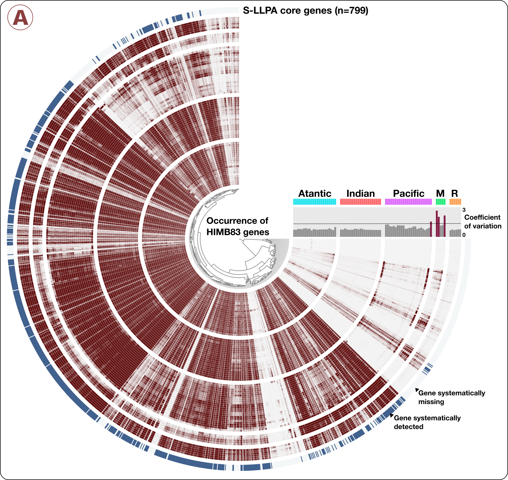
From the anvi’o metagenomic summary output described in the previous section, we determined the relative distribution of each genome across the 103 metagenomes. We created a text file, SAR11-PAN-samples-information.txt (avilable here) to link the pangenome to the environment using genomic coverage values across samples, as well as to display other information such as gneme lengths and clade information. From this file we generated an anvi’o samples database, SAR11-PAN-SAMPLES.db. In addition, we used the summary output of the SAR11 pangenome to identify protein clusters containing a list of HIMB83 genes of interest (the 799 core S-LLPA genes), and created the file S-LLPA-CORE-GENES.txt (avilable here), the contents of which looked like this:
$ head S-LLPA-CORE-GENES.txt
samples	S-LLPA_core_genes
PC_00000070	Yes
PC_00000046	Yes
PC_00000072	Yes
PC_00000079	No
PC_00000252	Yes
PC_00000176	Yes
PC_00000087	Yes
PC_00000043	Yes
PC_00000112	Yes
Finally, with all these additions, we visualized the SAR11 metapangenome:
anvi-display-pan -p SAR11-PAN-PAN.db \
                 -s SAR11-PAN-SAMPLES.db \
                 -g SAR11-GENOMES.h5 \
                 -A S-LLPA-CORE-GENES.txt
This resulting display is publicly available on the anvi-server just so you can play with it interactively in case you read it all the way here:
https://anvi-server.org/merenlab/sar11_metapangenome
doi:10.6084/m9.figshare.5248459 serves the anvi’o files for the SAR11 metapangenome.
Creating a self-contained profile for HIMB83
The 21 SAR11 genomes recruited more than one billion metagenomics reads, however we determined that one of these isolate genomes, HIMB83, was remarkably abundant and widespread across metagenomes and was of particular interest to study the genomic variability within the lineage represented by HIMB83 across geographies. To isolate HIMB83 from the rest of the data we used anvi-split, and created a self-contained anvi’o profile database for this genome.
Briefly, the program anvi-split creates a PROFILE subset of the merged PROFILE database so genomes of interest can be downloaded independently, and visualized interactively:
anvi-split -c SAR11-CONTIGS.db \
           -p SAR11-MERGED/PROFILE.db \
           -C Genomes \
           -b HIMB083 \
           -o SAR11-SPLIT-GENOMES
The resulting directory SAR11-SPLIT-GENOMES contains a subdirectory for HIMB83:
$ ls SAR11-SPLIT-GENOMES | head
HIMB083
$ ls NON-REDUNDANT-MAGs-SPLIT/HIMB083
AUXILIARY-DATA.h5.gz  CONTIGS.db  CONTIGS.h5  PROFILE.db
It is then possible to invoke the interactive interface and inspect reads this genome recruited across metagenomes using this command line:
anvi-interactive -c NON-REDUNDANT-MAGs-SPLIT/HIMB083/CONTIGS.db \
                 -p NON-REDUNDANT-MAGs-SPLIT/HIMB083/PROFILE.db
We finally run the summary of this bin;
anvi-summarize -p NON-REDUNDANT-MAGs-SPLIT/HIMB083/PROFILE.db \
               -c NON-REDUNDANT-MAGs-SPLIT/HIMB083/CONTIGS.db \
               -C DEFAULT \
               --init-gene-coverages \
               -o NON-REDUNDANT-MAGs-SPLIT/HIMB083/SUMMARY
doi:10.6084/m9.figshare.5248435 serves the self-contained anvi’o profile for HIMB83 across all metagenomes.
anvi-summarize allowed us to identity a list of 74 metagenomes where the mean coverage of HIMB83 was >50x. It is in these 74 metagenomes that we confidently detect HIMB83. We then identified 799 HIMB83 genes that systematically occurred in all 74 metagenomes (i.e. genes that were detected when HIMB83 was detected). Please see the methods section in our study for a more detailed description of these steps. But just to give a visual idea here, this shows the HIMB83 genes that systemmatically detected across metagenomes:
The files metagenomes-of-interest.txt and core-S-LLPA-genes.txt contain the names of of 74 metagenomes and gene caller id’s for 799 core genes, respectively. You can download these files into your work directory the following way:
curl -L -O http://merenlab.org/data/sar11-saavs/files/metagenomes-of-interest.txt
curl -L -O http://merenlab.org/data/sar11-saavs/files/core-S-LLPA-genes.txt
Quantifying the alignment quality of short reads to HIMB83 (and others)
It was of critical importance to quantify how well reads were mapping to HIMB83, as this gives some indication of what level of taxonomical group HIMB83 provides access to through read recruitment. The metric used to assess alignment quality was percent identity. A percent identity of 95% would mean that, for example, a 100 nucleotide-long read matched at 95 out of its 100 nucleotide positions to the reference sequence it aligned to. By calculating this for each read in a metagenome, the resulting histogram gives perspective on how similar the reads are to the reference.
To do this we wrote a python script that calculates a histogram for the percent identity of reads mapping to a reference genome. You should download the script:
curl -L -O http://merenlab.org/data/sar11-saavs/files/p-get_percent_identity.py
We used this script in a couple of different ways.
First, we calculated the percent identity histograms for each of the 21 isolates (over the whole genomes), where a metagenome was included for the isolate if the isolate’s coverage was >50X in that metagenome. A small directory outlining this information should be downloaded below:
curl -L -O http://merenlab.org/data/sar11-saavs/files/ALL_ISOLATES.zip
unzip ALL_ISOLATES.zip; rm ALL_ISOLATES.zip
The python script is then ran for each of these isolates. Please note that to simplify visualization of these distributions, only reads with lengths equal to the median read length were included and bins were defined so that each contains only one unique value. For example, if the median length was 100, the bins were defined like bin1 = (99%, 100%], bin2 = (98%, 99%], bin3 = (97%, 98%], etc. We allowed ourselves this freedom because we did not perform any statistical calculations with these distributions, as they were only generated for the purpose of visualization as a supplemental figure.
ls ALL_ISOLATES | while read isolate
do
    python p-get_percent_identity.py \
           -B ALL_ISOLATES/${isolate}/samples_with_greater_than_50_cov \
           -p \
           -R ALL_ISOLATES/${isolate}/contigs \
           -o PERCENT_IDENTITY_WHOLE_GENOME_${isolate}.txt \
           -range 65,100 \
           -autobin \
           -m \
           -melted \
           -interpolate 70,100,150
done
If you open up the script you’ll notice that it’s an absolute spaghetti monster, however it can accomplish a lot. If you want to see what the parameters do and change them for your own needs, pull up the help for the script:
python p-get_percent_identity.py -h
Second, we calculated the percent identity histograms for the 74 metagenomes in which HIMB83 recruited at least 50X coverage. Unlike in the previous command, in this case we focused to look only at the 799 core genes. We generated two outputs, one for visualization (which considers only reads with lengths equal to the median lengths and coarse bin sizes), and another that is statistically accurate (which takes into account all read lengths and has finely resolved bin sizes).
# Visualization purposes
python p-get_percent_identity.py \
       -B ALL_ISOLATES/HIMB083/samples_with_greater_than_50_cov \
       -p \
       -o PERCENT_IDENTITY_CORE_GENES_HIMB083_MEDIAN_LENGTH_ONLY.txt \
       -range 65,100 \
       -melted \
       -m \
       -autobin \
       -G core-S-LLPA-genes.txt \
       -a gene_calls_summary.txt \
       -interpolate 70,100,400 \
       -x

# Statistically rigourous
python p-get_percent_identity.py \
       -B ALL_ISOLATES/HIMB083/samples_with_greater_than_50_cov \
       -p \
       -o PERCENT_IDENTITY_CORE_GENES_HIMB083.txt \
       -range 65,100 \
       -numbins 4000 \
       -G core-S-LLPA-genes.txt \
       -a gene_calls_summary.txt \
       -x
Visualization of these distributions (for example Figure 2, Figure 4) reveal virtually all mapped reads share >88% read identity to HIMB83, which is significantly higher than the average nucleotide identity (ANI) between HIMB83 and HIMB122 (HIMB83’s closest isolated relative), ~82.5%.
Generating genomic variation data for HIMB83
To explore the genomic variability of 1a.3.V, the lineage recruited by HIMB83, we characterized SNVs and SAAVs for a set of HIMB83 genes across across metagenomes. Both for SNVs and SAAVs, we only considered positions of nucletides or codons that met a minimum coverage expectation. Controlling the minimum coverage of nucleotide or codon positions across metagenomes improves the confidence in variability analyses.
We generated three files to report the variability.
First we generated a report of SNVs in 799 genes across 74 metagenomes with a minimum departure from consensus value of 1%, and minimum nucleotide coverage across metagenomes value of 20x:
anvi-gen-variability-profile -c SAR11-CONTIGS.db \
                             -p SAR11-MERGED/PROFILE.db \
                             -C Genomes \
                             -b HIMB083 \
                             --samples-of-interest metagenomes-of-interest.txt \
                             --genes-of-interest core-S-LLPA-genes.txt \
                             --min-coverage-in-each-sample 20 \
                             --engine NT \
                             --quince-mode \
                             --min-departure-from-consensus 0.01 \
                             -o S-LLPA_SNVs_20x_1percent_departure.txt
Then we generated another report of SNVs in 799 genes across 74 metagenomes with a minimum departure from consensus value of 10%, and minimum nucleotide coverage across metagenomes value of 20x:
anvi-gen-variability-profile -c SAR11-CONTIGS.db \
                             -p SAR11-MERGED/PROFILE.db \
                             -C Genomes -b HIMB083 \
                             --samples-of-interest metagenomes-of-interest.txt \
                             --genes-of-interest core-S-LLPA-genes.txt \
                             --min-coverage-in-each-sample 20 \
                             --engine NT \
                             --quince-mode \
                             --min-departure-from-consensus 0.1 \
                             -o S-LLPA_SNVs_20x_10percent_departure.txt
And finally we generated a report of SAAVs for 799 genes across 74 metagenomes with a minimum departure from consensus value of 10%, and a minimum codon coverage across metagenomes of 20x:
anvi-gen-variability-profile -c SAR11-CONTIGS.db \
                             -p SAR11-MERGED/PROFILE.db \
                             -C Genomes \
                             -b HIMB083 \
                             --samples-of-interest metagenomes-of-interest.txt \
                             --genes-of-interest core-S-LLPA-genes.txt \
                             --min-coverage-in-each-sample 20 \
                             --engine AA \
                             --quince-mode \
                             --min-departure-from-consensus 0.1 \
                             -o S-LLPA_SAAVs_20x_10percent_departure.txt
These reports were the key data to compare the differential occurrence of variants across metagenomes to study the evolutionary forces operating on this lineage at large scale.
doi:10.6084/m9.figshare.5248447 serves the anvi’o variability tables described in this section.
Estimating the neutral AAST frequency distribution expectation
Bounds for the expected AAST frequency distribution assuming a neutral model were calculated in the following way. For rationalization of this approach, please refer to the methods section of the paper.
First, the frequency of codon usage was quantified throughout the 799 genes from the reference sequence.
anvi-get-codon-frequencies -c SAR11-CONTIGS.db -o codon_frequencies.txt
Next, the frequency distribution of expected AASTs based on the frequency of codons was calculated for both models: Model 1 in which the probability of double or triple mutations was zero, with a transition vs transversion rate of 2 (neutral_freq_dist_model_1.txt), and Model 2 where the probability of transitioning to any of the other 63 codons were equally probable, regardless of mutational distance or number of transitions/transversions (neutral_freq_dist_model_2.txt). Respectively, these distributions for the top 25 amino acids were calculated with the following commands:
curl -L -O http://merenlab.org/data/sar11-saavs/files/core-S-LLPA-genes.txt
curl -L -O http://merenlab.org/data/sar11-saavs/files/model_1_frequency_vector.py
curl -L -O http://merenlab.org/data/sar11-saavs/files/model_2_frequency_vector.py
python model_1_frequency_vector.py 2
python model_2_frequency_vector.py
Calculating allele frequency trajectories with respect to temperature
This brief section outlines how we made use of the SAAV table S-LLPA_SAAVs_20x_10percent_departure.txt to calculate allele frequency trajectories (illustrated in Figure S7) for each codon position that contained at least one SAAV. Allele frequency trajectories were calculated for each of such positions for the two amino acids comprising the most common AAST at that position. For example, if at some position, 40 of the 74 metagenomes had the AAST ‘alanine/serine’, and the remaining 34 metagenomes had the AAST ‘alanine/valine’, the trajectories of alanine and serine would be calculated. If in any of the metagenomes the coverage of both amino acids were 0, the position was discarded. For the remaining positions, the allele frequencies were correlated with in situ temperature with the script that can be downloaded like so:
curl -L -O http://merenlab.org/data/sar11-saavs/files/frequency_trajectories_dataset.py

# also download this guy
curl -L -O http://merenlab.org/data/sar11-saavs/files/TARA_metadata.txt
A table summarizing the results of a linear regression to temperature for each of these positions, i.e. Table S11, can then be generated with the command:
python frequency_trajectories_dataset.py --variability S-LLPA_SAAVs_20x_10percent_departure.txt -o allele_frequency_trajectory_summary.txt
SAAVs on protein structures
The workflow described below is now completely outdated and we highly recommend you use the workflow in this tutorial instead (http://merenlab.org/2018/09/04/structural-biology-with-anvio/) if you’re interested in protein structure prediction, as it simplifies things into just 2 anvi’o commands. For example, the entirety of what’s shown below could be accomplished with anvi-gen-structure-database -c SAR11-CONTIGS.db --genes-of-interest core-S-LLPA-genes.txt -o STRUCTURE.db followed by anvi-display-structure -p SAR11-MERGED/PROFILE.db -c SAR11-CONTIGS.db -s STRUCTURE.db.
The starting point for this section of the workflow is the SAAVs table for the core S-LLPA genes, which was generated in the “Generating genomic variation data for HIMB83” section as S-LLPA_SAAVs_20x_10percent_departure.txt.
Finding core S-LLPA genes with PDB matches
First, we BLAST searched 799 core S-LLPA genes against the Protein Data Bank (PDB) to determine which of them had sufficiently similar homologues with solved tertiary structure.
To do so we first created a FASTA file with amono acid sequences of the 799 genes,
# get all AA sequences in the contigs db
anvi-get-aa-sequences-for-gene-calls -c SAR11-CONTIGS.db -o SAR11-GENE-AA-SEQUENCES.fa

# subsample the core genes from it:
anvi-script-reformat-fasta SAR11-GENE-AA-SEQUENCES.fa
                           -I core-S-LLPA-genes.txt
                           -o CORE-S-LLPA-GENE-AA-SEQUENCES.fa
downloaded the PDB database as a single FASTA file,
curl -L -O ftp://ftp.wwpdb.org/pub/pdb/derived_data/pdb_seqres.txt.gz
gzip -d pdb_seqres.txt.gz
At the time of download for our study, the pdb_seqres.txt file was 125,199,982 bytes of data, although as of August 17th we note this has increased to 128,517,512 bytes. Since there is no version control with PDB data, new additions may yield slightly different results if you run our entire workflow, although we belive it is unlikely that the newly added protein sequences may influence the BLAST results.
created a BLAST database for PDB seqeunces,
makeblastdb -in pdb_seqres.fasta
            -dbtype prot
            -out pdb_seqres.fasta
and ran BLAST on the 799 genes:
blastp -query CORE-S-LLPA-GENE-AA-SEQUENCES.fa \
       -db pdb_seqres.fasta \
       -outfmt "6 qseqid sseqid pident qlen length mismatch gapopen qstart qend sstart send evalue bitscore" \
       -out CORE-S-LLPA-GENE-AA-SEQUENCES-vs-PDB-BLAST.fa
Next, we filtered out sequences with insufficient matches to the PDB. We accomplished this by considering only the PDB hit with the highest bitscore for each core S-LLPA gene, and by calculating proper_pident, which is the percentage of the query amino acids that were identical to an entry in the database given the entire lenght of the query sequence (so proper_pident helps us avoid the inflation of identity scores due to partial good matches). We filtered out genes in CORE-S-LLPA-GENE-AA-SEQUENCES.fa that had less than 30% proper_pident using the program anvi-script-filter-fasta-by-blast:
curl -L https://raw.githubusercontent.com/merenlab/anvio/master/sandbox/anvi-script-filter-fasta-by-blast -o anvi-script-filter-fasta-by-blast
chmod +x anvi-script-filter-fasta-by-blast
./anvi-script-filter-fasta-by-blast CORE-S-LLPA-GENE-AA-SEQUENCES.fa \
                                  --blast CORE-S-LLPA-GENE-AA-SEQUENCES-vs-PDB-BLAST.fa \
                                  --threshold 30 \
                                  --output-fasta CORE-S-LLPA-GENE-AA-SEQUENCES-W-PDB-MATCHES.fa \
                                  --outfmt "qseqid sseqid pident qlen length mismatch gapopen qstart qend sstart send evalue bitscore"
436 genes matched to these criteria are stored in CORE-S-LLPA-GENE-AA-SEQUENCES-W-PDB-MATCHES.fa for downstream analyses.
Protein structure prediction
We computationally predicted the protein structures of these 436 genes using a template-based tertiary structure prediction algorithm called RaptorX Structure Prediction. In short, RaptorX aligns query sequences to a database of solved protein structures, e.g. the PDB, and then uses the solved structures as templates to determine the conformation of the query sequence.
Using the submission form http://raptorx.uchicago.edu/StructurePrediction/predict/, we submitted protein structure prediction jobs in batches of 20 sequences (the limit imposed by RaptorX) by subdividing CORE-S-LLPA-GENE-AA-SEQUENCES-W-PDB-MATCHES.fa into 22 FASTA files.
RaptorX Structure Prediction outputs a zipped folder for each protein prediction named <sequence_id>.all_in_one.zip, where <sequence_id> is a unique tag generated by RaptorX. We created a new directory RaptorXProperty, manually moved all <sequence_id>.all_in_one.zip files into it, and unzipped them all. To make things more identifiable, we renamed the <sequence_id>.all_in_one folders to <corresponding_gene_call>.all_in_one, where <corresponding_gene_call> is the gene caller id defined by the SAAV table. To do this we created a python script called rename_all_in_ones.py, and executed it the following way:
curl -L -O http://merenlab.org/data/sar11-saavs/files/rename_all_in_ones.py
cd RaptorXProperty
python rename_all_in_ones.py
cd -
Before mapping SAAVs onto the predicted protein structure, we first did some maintenance on the SAAV table with the Python script curate_SAAV_table.py, which reads the original SAAV table S-LLPA_SAAVs_20x_10percent_departure.txt, and the ALL_SPLITS-gene_non_outlier_coverages.txt file that is generated when we summarized HIMB83 in the section “Creating a self-contained profile for HIMB83”.
# downlod the script
curl -L -O http://merenlab.org/data/sar11-saavs/files/curate_SAAV_table.py

# copy HIMB83 gene coverages from the summary dir (if you don't have this directory, the
# URL https://doi.org/10.6084/m9.figshare.5248435 serves HIMB83 profile with the SUMMARY
# output directory
cp NON-REDUNDANT-MAGs-SPLIT/HIMB083/SUMMARY/bin_by_bin/ALL_SPLITS/ALL_SPLITS-gene_non_outlier_coverages.txt .

# make sure the file S-LLPA_SAAVs_20x_10percent_departure.txt is also in this directory.
# if you don't have it, you may download the archive file that contains this and other files
# from the URL https://doi.org/10.6084/m9.figshare.5248447

# run the script
python curate_SAAV_table.py
Running this script will update the SAAV table with additional information, and create a new file called S-LLPA_SAAVs_20x_10percent_departure_curated.txt in the work directory.
Structural mapping of SAAVs
To map SAAVs onto protein structures, we developed a tool called SAAV-structural-mapping (https://github.com/merenlab/SAAV-structural-mapping) that visualizes SAAVs as spheres with different colors, sizes, and opacities. Each user-defined “perspective” defines how these three variables are controlled. Please visit the github page for instructions on how to install.
Unfortunately due to the limitations of PyMOL, SAAV-structural-mapping requires Python version 2, thus is not in the anvi’o codebase. We hope things will get better, and this step will be a part of the anvi’o codebase.
SAAV-structural-mapping depends on PyMOL, a molecular visualization package written in Python. For full functionality, a licensed version is required, however partial functionality is possible either with the free open-source version or the educational version (best alternative).
There are five inputs for this to work:
-
A gene list specifying the genes we are interested in visualizing. In the past we have visualized all of the 436 genes in the FASTA file (
CORE-S-LLPA-GENE-AA-SEQUENCES-W-PDB-MATCHES.fa), however the images require a lot of storage space and the script takes a very long time to run. To create the interface available at http://anvio.org/data/S-LLPA-SAAVs/, we subselected genes that looked visually interesting to us. If you have your own list of genes you’re interested in looking at, we encourage you to create your own gene list and let us know what you find! You can get a copy of ours this way: -
A TAB-delimited file with the first column specifying the samples we are interested in visualizing. We chose to only consider surface samples at a depth of 5m. The additional columns define how samples group together for the creation of multi-sample images. We grouped our samples based on region, main groups, and proteotypes. You can get a copy of our sample groups the following way:
-
A SAAV table. We used
S-LLPA_SAAVs_20x_10percent_departure_curated.txt. -
A collection of structure predictions for all the genes in
genes-of-interest-for-PyMOL.txt. We already created this: its theRaptorXPropertydirectory. -
A configuration file specifying how to visualize the SAAVs. Below is the configuration file we used (
structural-mapping-of-SAAVs-config.ini). For a complete description of how you can define your own config file please visit the help documentation of theanvi-map-saavs-to-structurescript in SAAV-structural-mapping.
You can get copies of missing files for a full analysis (gene list, samples mapping, and the configuration file) the following way:
curl -L -O http://merenlab.org/data/sar11-saavs/files/genes-of-interest-for-PyMOL.txt
curl -L -O http://merenlab.org/data/sar11-saavs/files/genes-of-interest-for-PyMOL.txt
curl -L -O http://merenlab.org/data/sar11-saavs/files/samples-of-interest-for-PyMOL.txt
For your information, our configuration file looked like this, and it is highly flexible for advanced users:
[BLOSUM90]
color_var = BLOSUM90
color_scheme = darkred_to_darkblue
merged_sphere_size_var = prevalence

[BLOSUM90_weighted]
color_var = BLOSUM90_weighted
color_scheme = darkred_to_darkblue
merged_sphere_size_var = prevalence

[solvent_accessibility]
color_var = solvent_acc
color_scheme = solvent_acc_cmap
merged_sphere_size_var = prevalence

[secondary_structure]
color_var = ss3
color_scheme = ss3_cmap
merged_sphere_size_var = prevalence

[AASTs]
color_var = competing_aas
color_scheme = competing_aas
merged_sphere_size_var = prevalence

[coverage_deviation]
color_var = rel_diff_from_mean_gene_cov
color_scheme = (#b6c7ee,#e8edf9,#ffffff,#fcf5f4,#7c0b03);(-0.94,-0.45,0.04,0.54,3.00)
merged_sphere_size_var = prevalence
With all of these pieces together, and assuming you did configure anvi-map-saavs-to-structure to be in your PATH, you can run the following command to generate output images:
pymol -r anvi-map-saavs-to-structure -- \
      --gene-list genes-of-interest-for-PyMOL.txt \
      --sample-groups samples-of-interest-for-PyMOL.txt \
      --saav-table S-LLPA_SAAVs_20x_10percent_departure_curated.txt \
      --input-dir RaptorXProperty \
      --pymol-config structural-mapping-of-SAAVs-config.ini \
      --ray 1 \
      --res 1200 \
      --output-dir SAR11-S-LLPA-SAAVs-ON-STRUCTURE
This will take some time. If you would like to speed it up, you can cut down on the number of perspectives in structural-mapping-of-SAAVs-config.ini and/or the number of genes in genes-of-interest-for-PyMOL.txt, and/or set --ray 0 and --res 600 for lower quality images.
The URL doi:10.5281/zenodo.835218 serves the output diretory, SAR11-S-LLPA-SAAVs-ON-STRUCTURE.
The output SAR11-S-LLPA-SAAVs-ON-STRUCTURE contains both PNG images for all the SAAV structure visualizations, as well as PyMOL files that can be opened to manipulate the structures.
Generating an interactive output
The resulting images with SAAVs mapped onto predicted tertiary structures of proteins can be neatly organized with functional annotation in an interactive interface with the following anvi’o command:
anvi-saavs-and-protein-structures-summary -i SAR11-S-LLPA-SAAVs-ON-STRUCTURE \
                                          -c SAR11-CONTIGS.db \
                                          -o S-LLPA-SAAVs \
                                          --soft-link-images \
                                          --perspectives 'AASTs,BLOSUM90,solvent_accessibility'
http://anvio.org/data/S-LLPA-SAAVs/ serves our S-LLPA-SAAVs output directory, which contains an interactive web page to explore 58 proteins across 49 samples with 3 perspectives in our config file.
The same output is also archived at doi:10.6084/m9.figshare.5248432.
Application of Deep Learning and Fixation Index to SAAVs
This section describes our use of deep learning to estimate distances between TARA metagenomes based on SAAVs identified in core S-LLPA genes. We used the resulting distance matrix to identify the main groups, and proteotypes displayed in Figure 3 in our study.
Setting the stage
Although it uses the SAAVs reported in the previous section, this part of our analysis is outside of anvi’o. To set the stage for this analysis, we first will create a Python 2.7 virtual environment and do some installation and configuration work. You can follow these steps to get everything ready:
# create a new python 2.7 virtual environment
virtualenv -p python2.7 ~/virtual-envs/LALNets

# activate it
source ~/virtual-envs/LALNets/bin/activate

# install tensorflow and Ozsel's LALNets library (while
# you're on it install ipython, too)
pip install tensorflow
pip install git+https://github.com/ozcell/LALNets.git
pip install ipython

# setup keras with theano backend
mkdir -p ~/.keras
cat << EOF >> ~/.keras/keras.json
{
    "image_dim_ordering": "tf",
    "epsilon": 1e-07,
    "floatx": "float32",
    "backend": "theano"
}
EOF
The rest of this section does two things: explaining the approach, and linking those explanations to Python code snippets, which you can run in a Python terminal (type ipython to start one). Alternatively, all steps are summarized in a single Python program at the end of this section, which you can run after making sure the path to the SAAVs table is correct. We are planning to implement this approach in anvi’o to streamline the application of this algorithm, but until then, you can use the following recipe.
These methods are adopted by our collaborators Ozsel Kilinc and Ismail Uysal. We thank them for their help with these analyses and for their patience :)
The approach
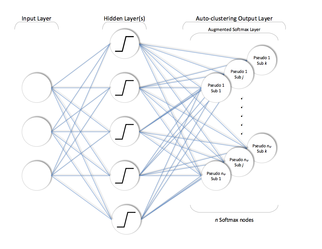
This approach builds upon a previous study on learning of latent annotations on neural networks using auto-clustering output layer (ACOL) when a coarse level of supervision is available for all observations (i.e. parent-class labels), but the model has to learn a deeper level of latent annotations (i.e. sub-classes, under each one of parents).
ACOL is a novel output layer modification for deep neural networks to allow simultaneous supervised classification (per provided parent-classes) and unsupervised clustering (within each parent) where clustering is performed with a recently proposed Graph-based Activity Regularization (GAR) technique. More specifically, as ACOL duplicates the softmax nodes at the output layer for each class, GAR allows for competitive learning between these duplicates on a traditional error-correction learning framework.
To study SAAVs, we modified ACOL to learn latent annotations in a fully unsupervised setup by substituting the real, yet unavailable, parent-class information with a pseudo one (i.e. randomly generated pseudo parent-classes). To generate examples for a pseudo parent-class, we choose a domain specific transformation to be applied to every sample in the dataset. The transformed dataset constitutes the examples of that pseudo parent-class and every new transformation (i.e. the random sampling of codon positions) generates a new pseudo parent-class. Naturally, the main classification task performed over these pseudo parent-classes does not represent any meaningful knowledge about the data by itself. However, frequent and random selection of these pseudo parent-classes allow the ACOL neural network to learn sub-classes of these pseudo parents without bias. While each sub-class corresponds to a latent annotation which may or may not be meaningful, the combination of these annotations learned through abundant and concurrent clusterings reveals an unbiased and robust similarity metric between different metagenomes.
Following sections describe the pseudo parent-class generation and similarity metric calculation along with the details of model training.
Loading the dataset
First we run all the import statements and read the anvi’o output for SAAVs into a Pandas dataframe:
from __future__ import print_function

import numpy as np
import pandas as pd

from keras.optimizers import SGD

from lalnets.commons.datasets import load_sar11
from lalnets.commons.utils import get_similarity_matrix
from lalnets.acol.models import define_mlp
from lalnets.acol.trainings import train_with_parents, get_model_truncated
from lalnets.metagenome.preprocessing import get_pseudo_labels_mini

np.random.seed(1337)

# path to the dataset:
loc = 'S-LLPA_SAAVs_20x_10percent_departure.txt'

#load the dataset
df, sample_id_map = load_sar11(loc)
Pseudo parent-class generation
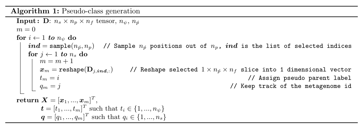
Consider an \(n_s \times n_p \times n_f\) metagenomics dataset represented by the 3-D tensor \(\mathbf{D}\), where \(n_s\) is the number of metagenomes to be clustered, \(n_p\) is the number of codon positions per metagenome and \(n_f\) is the number of features representing each codon position. Specifically, our dataset can be specified by a \(74 \times 37,416 \times 2\) tensor, as each codon position is represented by the two most frequent amino acids found in this position.
To generate the examples of \(i^{th}\) pseudo parent-class, we randomly sample \(n_{\acute{p}}\) positions out of \(n_p\) with replacement. Resulting \(n_s \times n_{\acute{p}} \times n_f\) subsets which correspond to \(d=n_{\acute{p}}n_f\) dimensional \(n_s\) examples of pseudo parent-class \(i\). This procedure is repeated for \(n_\psi\) times, and ultimately we obtain an \(m \times d\) input matrix \(\boldsymbol{X} = [\boldsymbol{x}_1,...,\boldsymbol{x}_{m}]^T\) and corresponding pseudo parent-class labels \(\boldsymbol{t}=[t_1,...,t_{m}]^T\) to train a neural network, where \(n_\psi\) is the number of the pseudo parents and \(m\) is the total number of the examples generated in this procedure, such that \(m=n_\psi n_s\).
We select \(n_{\acute{p}}=2000\) and \(n_\psi=1000\) to produce the results in this article, therefore \(\boldsymbol{X}\) is \(74000 \times 4000\) matrix where each one of 1000 pseudo parents is equally represented by 74 examples sampled from different metagenomes. We also keep track of the metagenome labels \(\boldsymbol{q}=[q_1,...,q_{m}]^T\), indicating the source metagenome of every example. This information will be used later to produce the similarity matrix.
Setting dataset paramters to set the stage for pseudo parent-class generation procedure:
# number of metagenomes
n_s = 74

# number of positions to be sampled
n_p_acute = 2000

# number of features per position
n_f = 2

# number of dimensions of the input
d = n_p_acute*n_f

# number of pseudo-classes
n_psi = 1000

# running the 'Algorithm 1: Pseudo-class generation':
X, t, q = get_pseudo_labels_mini(df, n_s, n_p_acute, n_psi)
The following describes the algorithm for sampling and pseudo parent-class generation procedure:
Learning Latent Annotations
Neural networks define a family of functions parameterized by weights and biases which define the relation between inputs and outputs. In multi-class categorization tasks, outputs correspond to class labels, hence in a typical output layer structure there exists an individual output node for each class. An activation function, such as softmax is then used to calculate normalized exponentials to convert the previous hidden layer’s activations, i.e. scores, into probabilities.
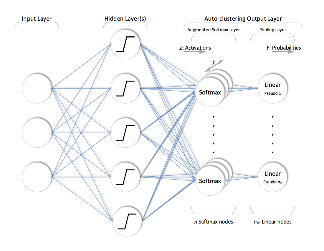
Unlike traditional output layer structure, ACOL defines more than one softmax node (\(k\) duplicates) per class (in this particular case, we prefer to use “pseudo parent-class” term to emphasize that these classes are not expert-defined but automatically generated depending on random sampling). Outputs of \(k\) duplicated softmax nodes that belong to the same pseudo parent are then combined in a subsequent pooling layer for the final prediction. Training is performed in the configuration shown in figure below. This might look like a classifier with redundant softmax nodes. However, duplicated softmax nodes of each pseudo parent are specialized due to dropout and the unsupervised regularization applied throughout the training in a way that each one of \(n=n_\psi k\) softmax nodes represents an individual sub-class of a pseudo parent, i.e. latent annotation.
Consider a neural network with ACOL consisting of \(L-1\) hidden layers where \(l\) denotes the individual index for each layer such that \(l \in \{0,...,L\}\). Let \(\boldsymbol{Y} ^{(l)}\) denote the output of the nodes at layer \(l\). \(\boldsymbol{Y} ^{(0)}=\boldsymbol{X}\) is the input and \(f(\boldsymbol{X})=f^{(L)}(\boldsymbol{X})=\boldsymbol{Y}^{(L)}=\boldsymbol{Y}\) is the output of the entire network, and \(\boldsymbol{W} ^{(l)}\) and \(\boldsymbol{b}^{(l)}\) are the weights and biases of layer \(l\), respectively. Then, the feedforward operation of the neural network can be written as
\[f^{(l)}\big(\boldsymbol{X}\big) = \boldsymbol{Y}^{(l)} = h^{(l)}\big(\boldsymbol{Y}^{(l-1)}\boldsymbol{W}^{(l)} + \boldsymbol{b}^{(l)}\big)\]where \(h^{(l)}\)(.) is the activation function applied at layer \(l\). For the sake of clarity, let’s specify the activities going into the augmented softmax layer of this network such that
\[\boldsymbol{Z} := \boldsymbol{Y}^{(L-2)}\boldsymbol{W}^{(L-1)} + \boldsymbol{b}^{(L-1)}\]and its positive part as \(\boldsymbol{B}\) such that
\[g\big(\boldsymbol{X}\big) = \boldsymbol{B} := \max{\big(\boldsymbol{0}, \boldsymbol{Z}\big)}\]both of which correspond to \(m \times n\) matrices, where \(n=n_\psi k\), and \(k\) is the clustering coefficient of ACOL (which we chose as 4 for our SAAVs data). The output of a neural network with ACOL can then be written in terms of \(\boldsymbol{Z}\) as
\[f\big(\boldsymbol{X}\big) = \boldsymbol{Y} = h^{(L)}\bigg(h^{(L-1)}\big(\boldsymbol{Z}\big)\boldsymbol{W}^{(L)} + \boldsymbol{b}^{(L)}\bigg)\]where \(\boldsymbol{Y}\) is an \(m \times n_\psi\) matrix in which \(Y_{ij}\) is the probability of the \(i^{th}\) example belonging to the \(j^{th}\) pseudo parent. Since \(h^{(L-1)}(.)\) and \(h^{(L)}(.)\) respectively correspond to softmax and linear activation functions and \(\boldsymbol{b}^{(L)} = \boldsymbol{0}\), then this expression further simplifies into
\[f\big(\boldsymbol{X}\big) = \boldsymbol{Y} = softmax\big(\boldsymbol{Z}\big)\boldsymbol{W}^{(L)}\]where \(\boldsymbol{W}^{(L)}\) is an \(n \times n_\psi\) matrix representing the constant weights between augmented softmax layer and pooling layer.
\[\boldsymbol{W}^{(L)}= \begin{bmatrix} \boldsymbol{I}_{n_\psi} \\ \boldsymbol{I}_{n_\psi} \\ \vdots \\ \boldsymbol{I}_{n_\psi} \end{bmatrix}\]and simply sums up the output probabilities of the softmax nodes belonging to the same pseudo-class. Since the output of the augmented softmax layer is already normalized, no additional averaging is needed at the pooling layer and summation alone is sufficient to calculate final pseudo-class probabilities. Also, unsupervised regularization \(\mathcal{U}(.)\) is applied to \(\boldsymbol{B}\) to penalize the range of its distribution. The overall objective function of the training then becomes
\[\mathcal{L}\big(\boldsymbol{Y}, \boldsymbol{t}\big) + \mathcal{U}\big(\boldsymbol{B}\big) = \mathcal{L}\big(softmax(\boldsymbol{Z})\boldsymbol{W}^{(L)}, \boldsymbol{t}\big) + c_R\sum\limits_{j=1}^{n}\bigg(\max\big(\boldsymbol{B}_{:,j}\big)-\min\big(\boldsymbol{B}_{:,j}\big)\bigg)\]where \(\mathcal{L}(.)\) is the supervised log loss function, \(\boldsymbol{t}=[t_1,...,t_{m}]^T\) is the vector of the provided pseudo parent labels such that \(t_i \in \{1,...,n_\psi\}\), \(\boldsymbol{B}_{:,j}\) corresponds to \(j^{th}\) column vector of matrix \(\boldsymbol{B}\) and \(c_R\) is the weighting coefficient.
We employ a neural network with 3 hidden layers of 2048 nodes,
# number of hidden layers, number of nodes per layer
mlp_params =(3, 2048)
and choose ACOL hyperparameters as follows:
# clustering coeffient of ACOL
k = 4

# dropout ratio to be applied to augmented softmax layer
p = 0.5

# weighting coeffient of the unsupervised regularization
c_R = 0.00001
Training of the newwork is performed according to simultaneous supervised and unsupervised updates resulting from the objective function given above. We adopt stochastic gradient descent in the mini-batch mode for optimization:
# define optimizer
sgd = SGD(lr=0.01, decay=1e-6, momentum=0.95, nesterov=True)
Algorithm 2 below describes the entire training procedure. Along with unsupervised regularization, it also applies dropout method to the augmented softmax layer to distribute examples across the duplicated softmax nodes. For each mini-batch, an \(1 \times n\) row vector \(\boldsymbol{r}\) of independent Bernoulli random variables is sampled and multiplied element-wise with the output of the augmented softmax layer. This operation corresponds to dropping out each one of the \(n\) softmax nodes with the probability of \(p\) for that batch.
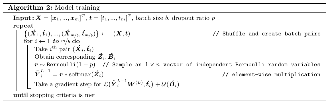
#Algorithm 2: Model training for 100 epochs
metrics, acti, model = train_with_parents(nb_parents = n_psi,
                                          nb_clusters_per_parent = k,
                                          define_model = define_mlp,
                                          model_params = model_params,
                                          optimizer = sgd,
                                          X_train = X,
                                          y_train = None,
                                          y_train_parent = t,
                                          X_test = X,
                                          y_test = None,
                                          y_test_parent = t,
                                          nb_reruns = 1,
                                          nb_epoch = 100,
                                          nb_dpoints = 10,
                                          batch_size = 128,
                                          test_on_test_set = False,
                                          update_c3 = None,
                                          return_model = True,
                                          save_after_each_rerun=None,
                                          model_in=None
                                          )
After training phase is completed, network is simply truncated by completely disconnecting the pooling layer as shown below.
The rest of the network with trained weights is used to assign the annotations to each example. This assignment can be described as
\[y_i := argmax_{1\le j \le n}Z_{ij}\]where \(y_i\) is the annotation assigned to \(i^{th}\) example.
#get assigned annotations
model_truncated = model.get_model_truncated(define_mlp, model_params, n_psi)
y = model_truncated.predict_classes(X, verbose=0)
Using the assigned annotations \(\boldsymbol{y}\) and the metagenome labels \(\boldsymbol{q}\), the similarity matrix \(\boldsymbol{S}\) used to obtain the dendrogram provided in this article is constructed as shown in Algorithm 3.
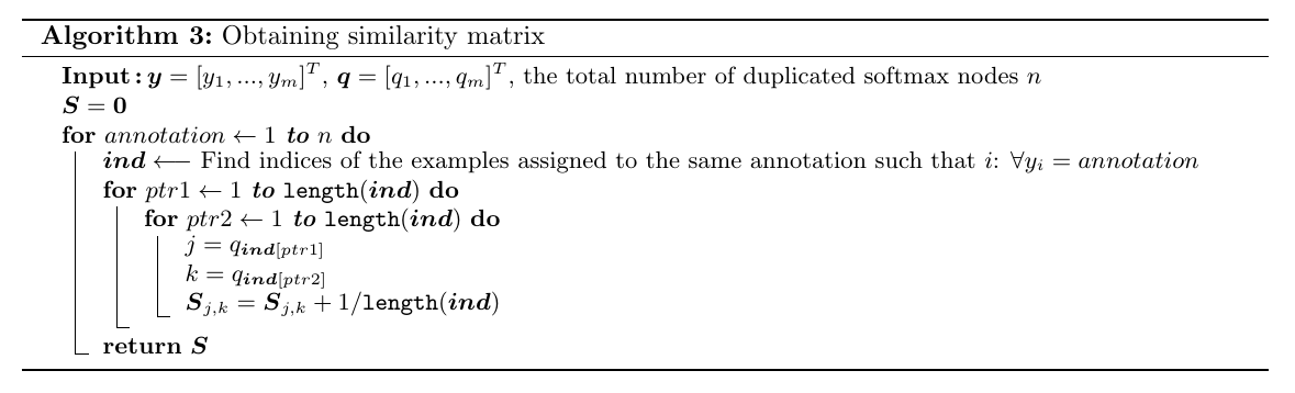
# Algorithm 3: Obtaining similarity matrix
_, S = get_similarity_matrix(q, y, n_psi, k, True)
Since applying dropout to distribute the examples across the duplicated softmax nodes also introduces a variance to the assigned annotations, we take the average of the similarity matrices obtained during the last 20 epochs of the training. Moreover, to reduce the variance due to the random generation of the pseudo parent-classes, we repeat the entire procedure 100 times with a new selection of pseudo parents for each repetition.
# Averaging hyperparameters for variance reduction
# number of epochs whose results to be averaged
n_avg = 20

# number of retrainings
n_exp = 100
The entire flow in Python
Assume the following code is stored in a file called ACOL_Pseudo_SAR11.py. We used the following code to obtain a matrix that describes pairwise distances between our metagenomes.
from __future__ import print_function

import numpy as np
import pandas as pd

from keras.optimizers import SGD

from lalnets.commons.datasets import load_sar11
from lalnets.commons.utils import get_similarity_matrix
from lalnets.acol.models import define_mlp
from lalnets.acol.trainings import train_with_parents, get_model_truncated
from lalnets.metagenome.preprocessing import get_pseudo_labels_mini

# set seed for reproducibility
np.random.seed(1337)

# path of the dataset
loc = 'S-LLPA_SAAVs_20x_10percent_departure.txt'

# load the dataset
df, sample_id_map = load_sar11(loc)

# Dataset hyperparameters ######################################
n_s = 74 # num metagenomes
n_p_acute = 2000 # num positions to be sampled
n_f = 2 # num features per position
n_psi = 1000 # num pseudo-classes
d = n_p_acute*n_f # num dimensions of the input
#################################################################

# NN hyperparameters ############################################
mlp_params =(3, 2048) # num hidden layers & num nodes per layer
#################################################################

# ACOL hyperparameters ##########################################
k = 4 # clustering coeffient of ACOL
p = 0.5 # dropout ratio to be applied to augmented softmax layer
c_R = 0.00001 # weighting coeff. of the unsuperv. regularization
#################################################################

# define model
acol_params = (k, p, c_R, None, None, None, 0, 'average', False)
model_params = ((d,), n_psi, mlp_params, (0., 0., 2.), True, acol_params)

# define optimizer
sgd = SGD(lr=0.01, decay=1e-6, momentum=0.95, nesterov=True)

# number of epochs whose results to be averaged
n_avg = 20

# number of retrainings
n_exp = 100

# initialize similarity matrices
S_avg = np.zeros((n_s, n_s, n_avg))
S_all = np.zeros((n_s, n_s, n_exp))

for exp in range(n_exp):
    # Algorithm 1: Pseudo-class generation
    X, t, q = get_pseudo_labels_mini(df, n_s, n_p_acute, n_psi)

    # Algorithm 2: Model training for 100 epochs
    metrics, acti, model = train_with_parents(nb_parents = n_psi,
                                              nb_clusters_per_parent = k,
                                              define_model = define_mlp,
                                              model_params = model_params,
                                              optimizer = sgd,
                                              X_train = X,
                                              y_train = None,
                                              y_train_parent = t,
                                              X_test = X,
                                              y_test = None,
                                              y_test_parent = t,
                                              nb_reruns = 1,
                                              nb_epoch = 100,
                                              nb_dpoints = 10,
                                              batch_size = 128,
                                              test_on_test_set = False,
                                              update_c3 = None,
                                              return_model = True,
                                              save_after_each_rerun=None,
                                              model_in=None
                                              )

    # train the model for n_avg more epochs
    for i in range(n_avg):
        # Algorithm 2: Model training for 1 epoch
        metrics, acti, model = train_with_parents(nb_parents = n_psi,
                                                  nb_clusters_per_parent = k,
                                                  define_model = define_mlp,
                                                  model_params = model_params,
                                                  optimizer = sgd,
                                                  X_train = X,
                                                  y_train = None,
                                                  y_train_parent = t,
                                                  X_test = X,
                                                  y_test = None,
                                                  y_test_parent = t,
                                                  nb_reruns = 1,
                                                  nb_epoch = 1,
                                                  nb_dpoints = 1,
                                                  batch_size = 128,
                                                  test_on_test_set = True,
                                                  update_c3 = None,
                                                  return_model = True,
                                                  save_after_each_rerun=None,
                                                  model_in=model
                                                  )

        # get assigned annotations
        model_truncated = model.get_model_truncated(define_mlp, model_params, n_psi)
        y = model_truncated.predict_classes(X, verbose=0)

        # Algorithm 3: Obtaining similarity matrix
        _, S = get_similarity_matrix(q, y, n_psi, k, True)
        S_avg[:,:,i] = S

    # take the average of the similarity matrices obtained during last n_avg epochs
    S_all[:,:,exp] = S_avg.mean(axis=-1)

# take the average of all similarity matrices obtained in n_exp retrainings
S = S_all.mean(axis=-1)
df_S = pd.DataFrame(S, index=sample_id_map)

# report the distance matrix
df_S.to_csv('S-LLPA-DEEP-LEARNING-DIST-MAT.csv', header=True, index=True, sep='\t')
This will run orders of magnitude faster When a cuda enabled GPU is available on the machine. In which case you can run it this way:
export THEANO_FLAGS=mode=FAST_RUN,device=gpu,lib.cnmem=0.95,floatX=float32
python ACOL_Pseudo_SAR11.py
otherwise you can run it this way:
export THEANO_FLAGS=mode=FAST_RUN,device=cpu,lib.cnmem=0.95,floatX=float32
python ACOL_Pseudo_SAR11.py
Running this code generates the TAB-delimited output file S-LLPA-DEEP-LEARNING-DIST-MAT.csv which contains deep learning-estimated distances between metagenomes. A copy of this distance matrix is available here.
Generating distance matrices from fixation index for SAAVs and SNVs data
As well as deep learning, we also attempted to cluster the SAAVs and SNVs using fixation index, the workflow to generate distance matrices is described here:
anvi-gen-fixation-index-matrix -V S-LLPA_SNVs_20x_1percent_departure.txt -o NT_fixation_indices.txt --engine NT
anvi-gen-fixation-index-matrix -V S-LLPA_SAAVs_20x_10percent_departure.txt -o AA_fixation_indices.txt --engine AA
anvi-matrix-to-newick NT_fixation_indices.txt
anvi-matrix-to-newick AA_fixation_indices.txt
A copy of the SAAVs data distance matrix is available here in the SNVs data distance matrix here.
Identifying proteotypes from Deep Learning and Fixation Index Distances
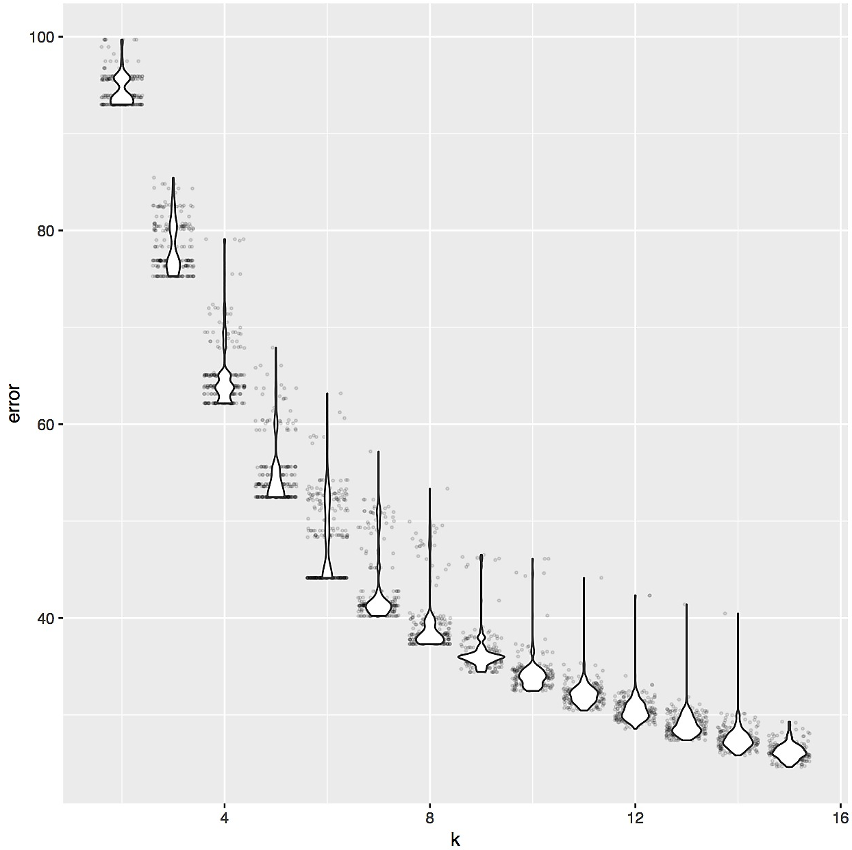
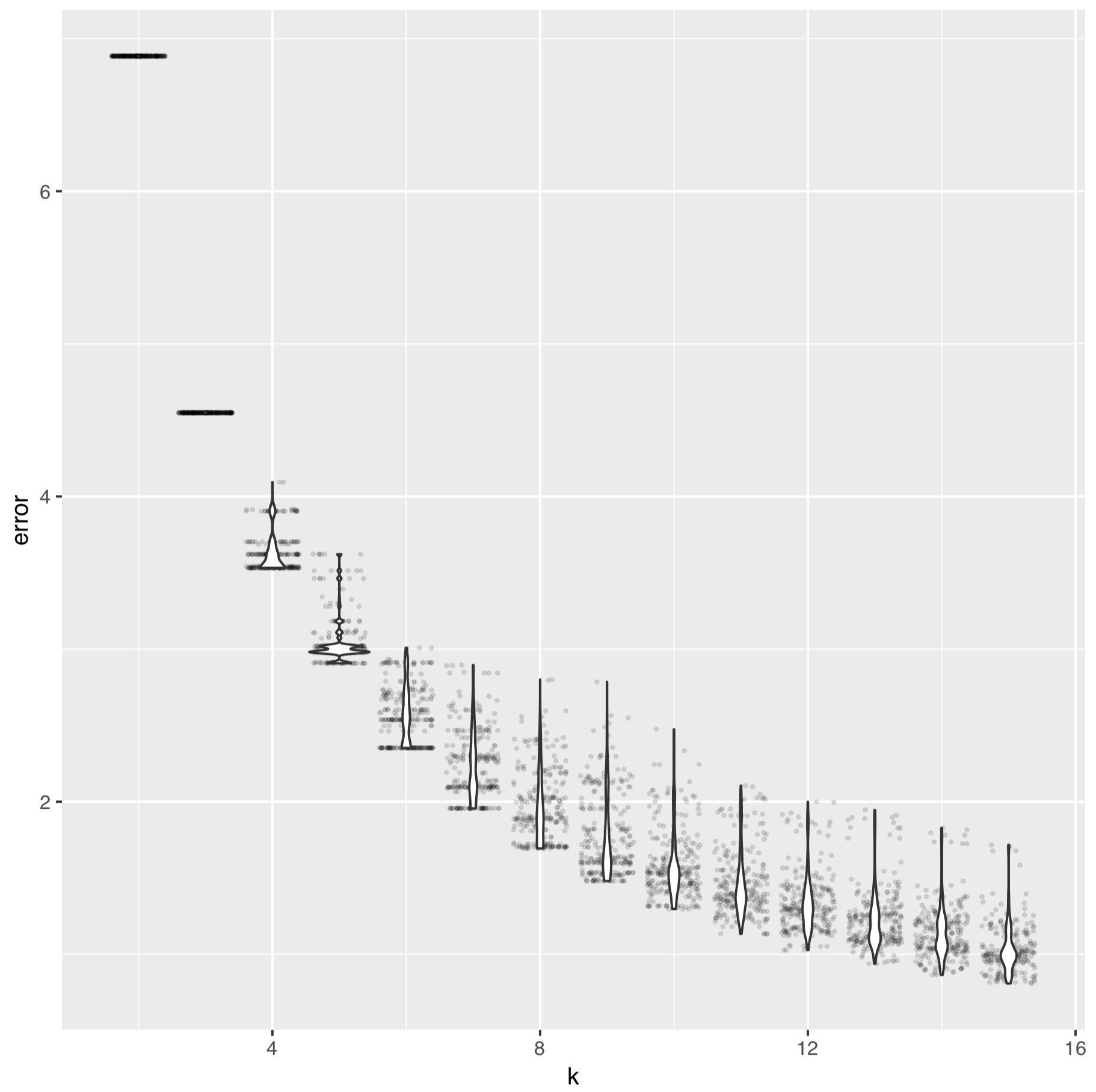
The distance matrix S-LLPA-DEEP-LEARNING-DIST-MAT.csv contained distances across metagenomes, from which we could obtain a hierarchical clustering of our metagenomes. Yet, the identification of proteotypes required us to cut this dendrogram into a reasonable number of sub-clusters. To determine the appropriate number, we relied on the elbow of the intra-cluster sum-of-squares curve of k-means by running the following R code on the S-LLPA-DEEP-LEARNING-DIST-MAT.csv,
#!/usr/bin/env Rscript
# Visualize the squared mean error per number of k-means clusters given a distance matrix

library(ggplot2)

deep_learning_dists <- read.table("S-LLPA-DEEP-LEARNING-DIST-MAT.csv", sep=",", header=TRUE, row.names=1)

df <- data.frame(k=numeric(), error=numeric())

for (i in 1:250){
  for (j in 2:15){
    df <- rbind(df, c(j, sum(kmeans(deep_learning_dists, centers=j)$withinss)))
  }
}

names(df) <- c('k', 'error')

pdf('./num_clusters.pdf')
ggplot(df, aes(x=k, y=error, group=k)) + geom_jitter(alpha=0.1, size=0.5) + geom_violin()
dev.off()
which suggested that ‘six’ was an appropriate number to divide our dendrogram:
We also applied the same clustering of samples based on fixation index for both the SAAV data and the SNVs data using an almost identical script:
#!/usr/bin/env Rscript
# Visualize the squared mean error per number of k-means clusters given a distance matrix

library(ggplot2)

AA_fixation_index_dists <- read.table("AA_fixation_indices.txt", sep="\t", header=TRUE, row.names=1)
NT_fixation_index_dists <- read.table("NT_fixation_indices.txt", sep="\t", header=TRUE, row.names=1)

AA_df <- data.frame(k=numeric(), error=numeric())
NT_df <- data.frame(k=numeric(), error=numeric())

for (i in 1:250){
  for (j in 2:15){
    AA_df <- rbind(AA_df, c(j, sum(kmeans(AA_fixation_index_dists, centers=j)$withinss)))
    NT_df <- rbind(NT_df, c(j, sum(kmeans(NT_fixation_index_dists, centers=j)$withinss)))
  }
}

names(AA_df) <- c('k', 'error')
names(NT_df) <- c('k', 'error')

pdf('./num_clusters_AA_fixation_index.pdf')
ggplot(AA_df, aes(x=k, y=error, group=k)) + geom_jitter(alpha=0.1, size=0.5) + geom_violin()
dev.off()

pdf('./num_clusters_NT_fixation_index.pdf')
ggplot(NT_df, aes(x=k, y=error, group=k)) + geom_jitter(alpha=0.1, size=0.5) + geom_violin()
dev.off()
The elbow of the intra-cluster sum-of-squares curve of k-means of fixation indices of the SNV data looks like:
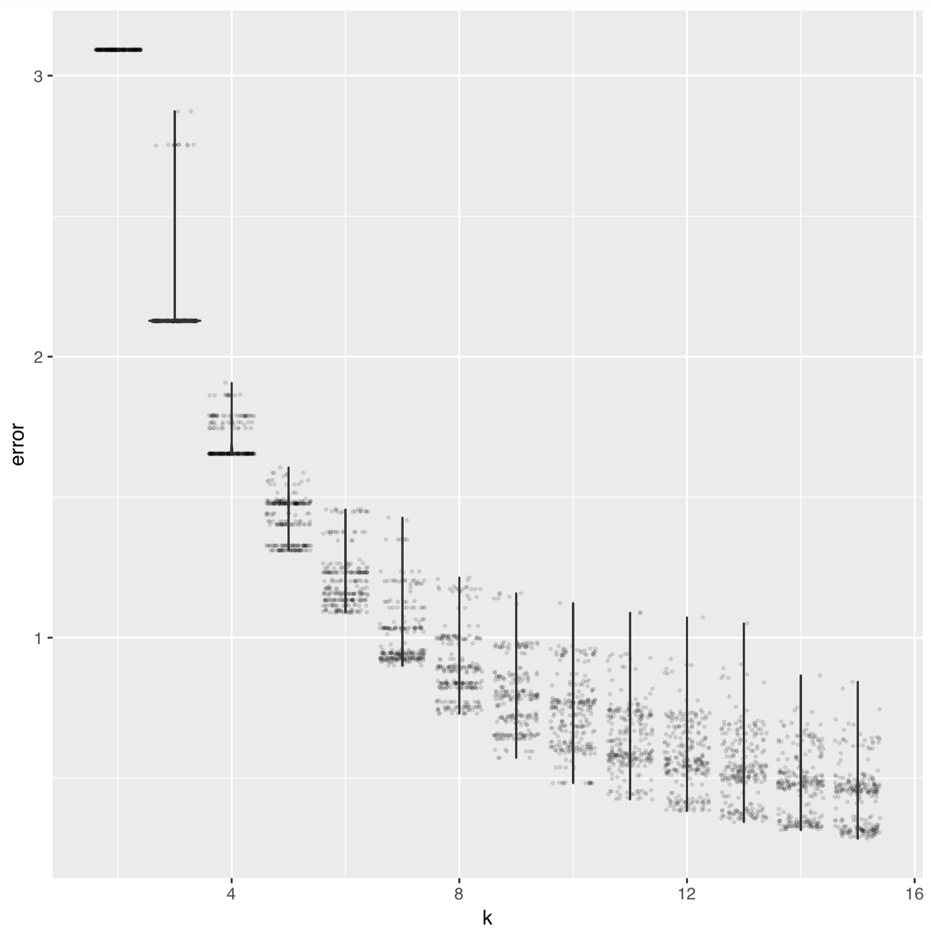
And for the SAAV data it looks like:
References
-
Eddy SR. (2011). Accelerated Profile HMM Searches. PLoS Comput Biol 7: e1002195.
-
Eren AM, Esen ÖC, Quince C, Vineis JH, Morrison HG, Sogin ML, et al. (2015). Anvi’o: an advanced analysis and visualization platform for ‘omics data. PeerJ 3: e1319.
-
Eren AM, Vineis JH, Morrison HG, Sogin ML. (2013). A Filtering Method to Generate High Quality Short Reads Using Illumina Paired-End Technology. PLoS One 8: e66643.
-
Hyatt D, Chen G-L, Locascio PF, Land ML, Larimer FW, Hauser LJ. (2010). Prodigal: prokaryotic gene recognition and translation initiation site identification. BMC Bioinformatics 11: 119.
-
Langmead B, Salzberg SL. (2012). Fast gapped-read alignment with Bowtie 2. Nat Methods 9: 357–359.
-
Li H, Handsaker B, Wysoker A, Fennell T, Ruan J, Homer N, et al. (2009). The Sequence Alignment/Map format and SAMtools. Bioinformatics 25: 2078–2079.
-
Minoche AE, Dohm JC, Himmelbauer H. (2011). Evaluation of genomic high-throughput sequencing data generated on Illumina HiSeq and genome analyzer systems. Genome Biol 12: R112.
-
Sunagawa S, Coelho LP, Chaffron S, Kultima JR, Labadie K, Salazar G, et al. (2015). Ocean plankton. Structure and function of the global ocean microbiome. Science 348: 1261359.
-
Kopf, A., M. Bicak, and R. Kottmann. The ocean sampling day consortium. GigaScience. 2015; 4: 27.