Studying hypervariability in genomes through metagenomes


Table of Contents
- Introduction
- Downloading the genome
- Downloading the metagenomes
- The metagenomic read recruitment
- Taking an initial look at the read recruitment results
- Looking for RTs in the genome
- Visualizing coverage and single-nucleotide variants (SNVs)
- Working with single-amino acid variants (SAAVs)
- Defining an in silico primer and collecting reads
- Performing an oligotyping analysis
Summary
The purpose of this tutorial is to demonstrate a bioinformatics workflow that enables the use of metagenomics to recognize hypervariable regions in microbial genomes and helps quantify and characterize the within-population sequence diversity of such regions for ecological and evolutionary surveys of naturally ocurring mirobial populations.
While this tutorial uses diversity-generating retroelements (DGRs) as an example and focuses on the activity of a particular DGR in a Trichodesmium genome, the strategies covered in this document are applicable to any other context in which rampant hypervariability or subtle microdiversity is of interest.
The tutorial also serves as a reproducible bioinformatics workflow for the recent review Blair Paul and I wrote on some of the most beautiful and mysterious ways for life to beat the boring means of evolution and skip ahead:
The organization of the document will follow the organization of Figure 3 in that work, and will demonstrate the key analysis steps that led to its emergence. We hope that this workflow will inspire you to keep in mind,
- The importance of studying metagenomic coverage data more carefully,
- The utility of single-nucleotide variants (SNVs) to recognize biological phenomena,
- The power of single-amino acid variants (SAAVs) to quantify non-synonymous variation,
- The ways to access unmapped or unmappable but critically relevant metagenomic short reads that originate from hypervariable regions through in silico primers,
- The application of oligotyping to metagenomics to investigate the nexus between ecology and hypervariability,
- The integrated platform anvi’o for similar novel investigations for which there are no off-the-shelf software options or canned solutions.
Introduction
This tutorial will walk you through a high-resolution approach to study within-population sequence diversity of environmental microbes in the context of short genomic regions using metagenomics.
Microbiology is drowning in publicly available ‘omics data from any habitat. Yet, even though the computational strategies to study such data are most powerful in the hands of life scientists, it is still a challenge to take the initial steps into the world of ‘omics. While many off-the-shelf tools for metagenomics conveniently take in raw data and produce final outuputs, the ability to control what happens in between remains to be a luxury that only computational folk can afford. But some questions of microbiology require much more hands-on access and control over complex data than others. I believe sudying hypervariability or microdiversity are two of such questions where it is very difficult to get meaningful answers from automated approaches. The good news is that making sense of hypervariability using complex data sources without any expertise in computation AND without having to use any black-box automation is not impossible. This tutorial aims to serve as an example to that statement by walking you through a singular path as it dives into a simple question. I hope while going through this random walk you will also see the forest and recognize other potential directions that may take you to more relevant places for your own data analyses since computational strategies covered here will be most useful to life scientists who wish to have full control over their data to conduct meticulous and hands-on analyses.
If you wish to conduct similar analyses to those you will see in this document, all you need is a genome of your favorite organism, and some metagenomes in which you expect populations that match to your organism to be relatively abundant. If any of the following sections confuse you, please feel free to leave a comment down below or get in touch with Blair Paul or Meren to bounce ideas.
Most of the bioinformatics on this page will use anvi’o, a community-led, integrated, reproducible software platform for multi-omics. If you have everything you need and interested in using anvi’o, but you are not sure which anvi’o programs and artifacts would help you best conduct your investigation, please reach out to the anvi’o community via Discord:

As I mentioned, one of the major goals of this tutorial is to share the bioinformatics steps that led to the emergence of this figure,
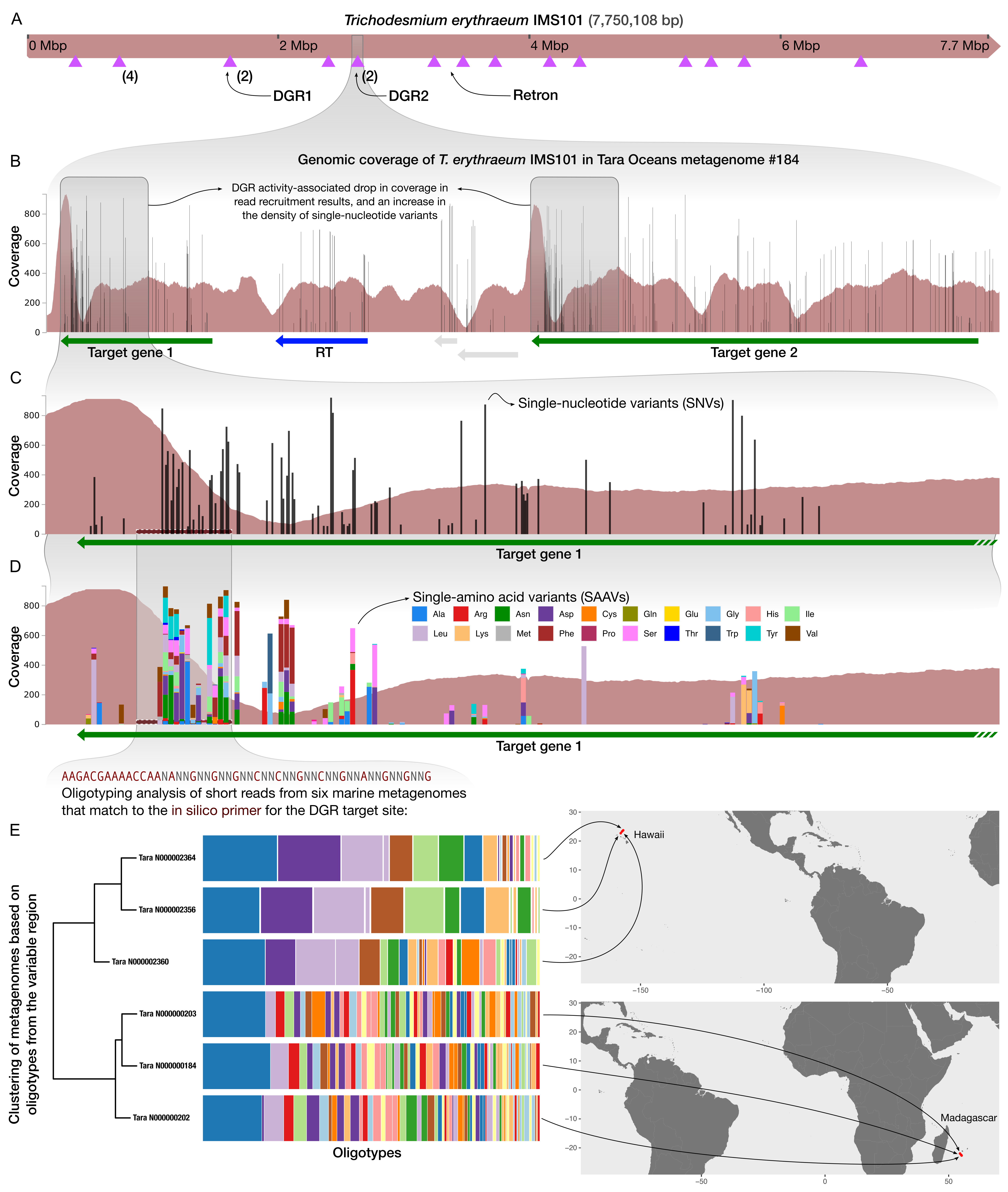
in which,
- Panel A shows a sketch of a microbial genome, indicating the locations of several DGRs and target genes as well as a retron (purple triangles),
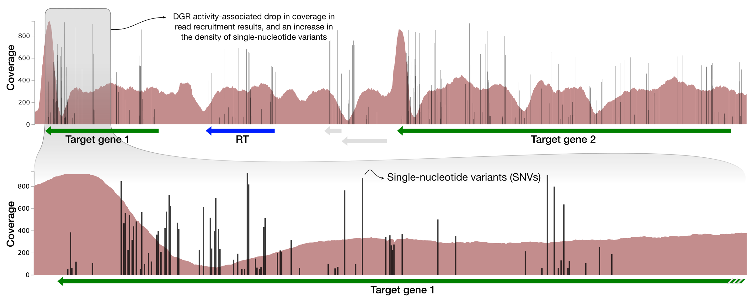
- Panel B visualizes the results of a metagenomic read recruitment analysis, and in particular the coverage of a particular genomic region that contains some genes of interest,
- Panel C details the drop in coverage and increase in the density of single-nucleotide variants (SNVs) in Target Gene 1,
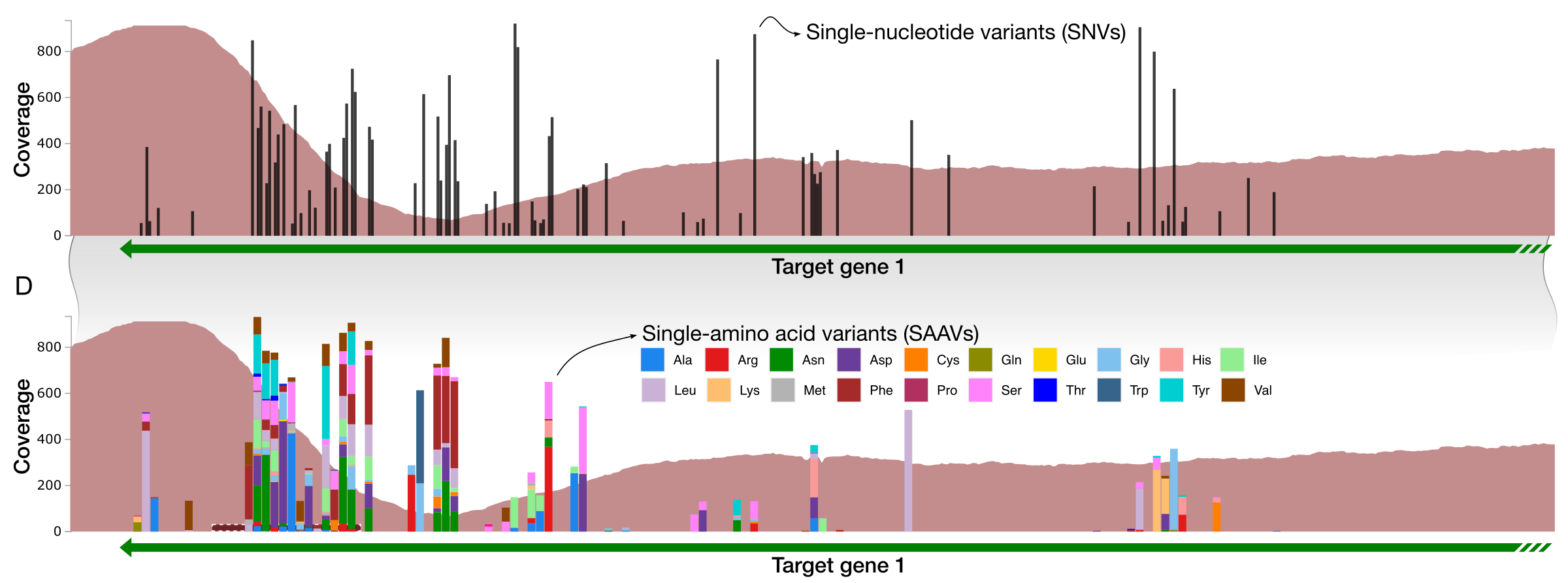
- Panel D visualizes single-amino acid variants (SAAVs) in the same region, and finally,
- Panel E describes an oligotyping analysis of the metagenomic short reads that are recovered from the raw FASTQ files using an ‘in silico primer’, to discuss the ecological signal in this hypervariable region.
If you are here, it is more likely than not that you can name a genome of your interest and a resource for metagenomic data to investigate it. But I will assume that you may not be as familiar with the general strategies or concepts mentioned in the list above (i.e., metagenomics, SNVs, SAAVs, etc.), and I will try to detail them throughout. Please feel free to send an email if you think something deserves to be detailed further.
To demonstrate ways to study hypervariable genomic regions through metagenomics, Blair and I decided to use Trichodesmium erythraeum IMS101 as our genome and one of its diveristy-generating retroelements, and some marine metagenomes made available by the Tara Oceans Project to make sense of environmental populations of Trichodesmium erythraeum.
Diversity-generating retroelements (DGRs) was a good choice to study hypervariability, since they represent one of the most fascinating genetic mechanisms through which bacteria and archaea can diversity their proteins in astonishing speeds. Trichodesmium erythraeum was a good choice, too, thanks to the literature on this organism and other cyanobacteria by Ulrike Pfreundt et al (2014) as well as Alec Vallota-Eastman et al (2020). But as you can imagine, everything here will work as effectively if you were to use a Bacteroides fragilis genomes and some human gut metagenomes.
If you are interested in reproducing this tutorial, please consider installing anvi’o first.
Downloading the genome
First things first: the genome. We downloaded a genome for the T. erythraeum IMS101 strain through this page on NCBI. Just for posterity, here is the FASTA file that we ended up working with:
Downloading the metagenomes
Second, we need metagenomes to chracterize environmental populations of T. erythraeum. So we downloaded the following six metagenomes from the collection of Tara Oceans Project metagenomes:
| Tara Sample | Station | Region | Lat | Lon | Depth (m) |
|---|---|---|---|---|---|
| TARA_N000000184 | TARA_051 | [IO] Indian Ocean | -21,4593 | 54,3041 | 5,97 |
| TARA_N000000202 | TARA_051 | [IO] Indian Ocean | -21,5043 | 54,3563 | 5,97 |
| TARA_N000000203 | TARA_051 | [IO] Indian Ocean | -21,5043 | 54,3563 | 5,97 |
| TARA_N000002356 | TARA_131 | [NPO] North Pacific Ocean | 22,7091 | -158,0247 | 5,88 |
| TARA_N000002360 | TARA_131 | [NPO] North Pacific Ocean | 22,7267 | -157,9955 | 5,88 |
| TARA_N000002364 | TARA_131 | [NPO] North Pacific Ocean | 22,7511 | -157,9632 | 5,88 |
Let’s first address why this particular six when there are many more marine metagenomes by Tara Oceans Project, and not all of them.
We chose this particular set because we initially determined in which Tara Oceans metagenomes T. erythraeum IMS101 had the highest coverage. Hypervariability is the enemy of coverage, and everything we will do downstream will work best if the coverage of a given genome is, on average, more than 50X in a given metagenome. This may be too conservative for some analyses, and one can survive with much less coverage, but as the coverage goes down, our confidence will go down with it.
To keep things simple, I will not go into the details of the initial steps of the analysis to identify which six metagenomes to use, but they are nothing more than doing read recruitment using all metagenomes, and then quickly profiling them, for which using a program like anvi-profile-blitz) can be extremely time-effective. But let’s forget about it for now, and talk about the next step. Finally, while I’m here, I thank Matt Schechter for his help downloading all the Tara Oceans Project metagenomes for the large size fraction!
The metagenomic read recruitment
If you are not familiar with metagenomic read recruitment, let’s start from here: it is the most essential first step for the vast majority of studies that make use of metagenomics. If you would like to familiarize yourself with terms and concepts in metagenomic read recruitment, you can watch this introductory video that will offer you a quick and easy introduction to its fundamentals:
In addition, you can go through this tutorial to have some idea about how key steps of actually performing metagenomic read recruitment looks or feels like.
But if you would like to follow this document a little longer, this is how my work directory looked like this after downloading the genome and metagenomes, which are all the files we need to perform a metagenomic read recruitment analysis.
$ ls

T_erythraeum_IMS101.fa
ERR1726621_1.fastq.gz
ERR1726621_2.fastq.gz
ERR1726854_1.fastq.gz
ERR1726854_2.fastq.gz
ERR1726640_1.fastq.gz
ERR1726924_1.fastq.gz
ERR1726640_2.fastq.gz
ERR1726924_2.fastq.gz
ERR1726697_1.fastq.gz
ERR1726697_2.fastq.gz
ERR1726823_1.fastq.gz
ERR1726823_2.fastq.gz
ERR1726921_1.fastq.gz
ERR1726921_2.fastq.gz
Careful readers will notice that there are 7 pairs of R1 and R2 files for six metagenomes, rather than 12. This is the case in this particular instance because one of the metagenomes was sequenced multiple times, hence the two extra files.
In theory what we will do with our T. erythraeum IMS101 genome and six Tara Oceans Project metagenomes is not any different at all than what is explained in the metagenomics read-recruitment tutorial and the steps covered in it. You may very well perform your own read recruitment analyses for your genomes and metagenomes following that tutorial alone, and get two primary anvi’o data products that we will use for everything downstream: contigs-db and profile-db. So, doing the read recruitment manually is the option one.
But if you have hundreds of metagenomes, or if you want to use a high-performance computing system to do the job for you, doing these steps manually does not scale well (even though it certainly is the best to do at least a few manual metagenomic read recruitment analyses just to familiarize yourself with all the steps first). For this reason, and for the sake of reproducibility, our group exclusively uses anvi’o snakemake workflows for read recruitment analyses, which help us automatize all the rudimentary steps to get our anvi’o contigs-db and profile-db, magical files the utility of which are hopefully going to be clearer to you as you go through the rest of this document. So, doing the read recruitment automatically is the option two.
If you were to go with the option two, and follow the tutorial for anvi’o snakemake workflows, you would realize that if you have a genome and a bunch of metagenomes to recruit reads from, we would need to use what is called the metagenomics workflow in reference mode (where the reference is the genome you already have, in contrast to the ‘default mode’ where anvi’o would first assemble your metagenomes and use the resulting contigs to do the read recruitment). The same tutorial would also tell you that to run the metagenomics workflow in reference mode, one would need a fasta-txt file and a samples-txt file to describe their data neatly. The fasta-txt for this analysis looked like this,
| name | path |
|---|---|
| T_erythraeum_IMS101 | T_erythraeum_IMS101.fa |
and the samples-txt file looked like this:
| sample | r1 | r2 |
|---|---|---|
| TARA_N000002360 | ERR1726621_1.fastq.gz | ERR1726621_2.fastq.gz |
| TARA_N000000202 | ERR1726854_1.fastq.gz | ERR1726854_2.fastq.gz |
| TARA_N000002356 | ERR1726640_1.fastq.gz,ERR1726924_1.fastq.gz | ERR1726640_2.fastq.gz,ERR1726924_2.fastq.gz |
| TARA_N000000184 | ERR1726697_1.fastq.gz | ERR1726697_2.fastq.gz |
| TARA_N000002364 | ERR1726823_1.fastq.gz | ERR1726823_2.fastq.gz |
| TARA_N000000203 | ERR1726921_1.fastq.gz | ERR1726921_2.fastq.gz |
Once you have these two TAB-delimited files ready, running the metagenomics workflow is just a single command line using the program anvi-run-workflow. We did it, and made the resulting anvi’o databases publicly available at 10.6084/m9.figshare.17708678.
Taking an initial look at the read recruitment results
Regardless of the path you have followed, if you are here, this document assumes that you have your contigs-db and profile-db files ready.
If you do not have them, but still would like to reproduce the rest of the steps in this document, you can download the files that we used for our analysis by typing the following commands in your terminal on your anvi’o installed computer:
# download the reproducible data pack
curl -L https://cloud.uol.de/public.php/dav/files/5p6iE4qegNDZ2mY \
     -o TRICHO-DGRs.tar.gz

# unpack the data pack
tar -zxvf TRICHO-DGRs.tar.gz

# go into the new directory
cd TRICHO-DGRs
The rest of this workflow will assume when you type ls in your work directory, you see the following files, which correspond to our copies of the contigs-db (the file named CONTIGS.db) and profile-db (the file named PROFILE.db):
AUXILIARY-DATA.db CONTIGS.db PROFILE.db
The AUXILIARY-DATA.db file is also an anvi’o artifact, but essentially it is automatically generated by anvi-merge as an accessory (albeit a critical one) to the PROFILE.db, so we never mention it even though you also need to have that file in your work directory.
If you have these files accessible to you, then you should be able to take a first look at the read recruitment results with anvi-interactive by running the following command,
anvi-interactive -p PROFILE.db -c CONTIGS.db
which should open your browser to present you with this display:
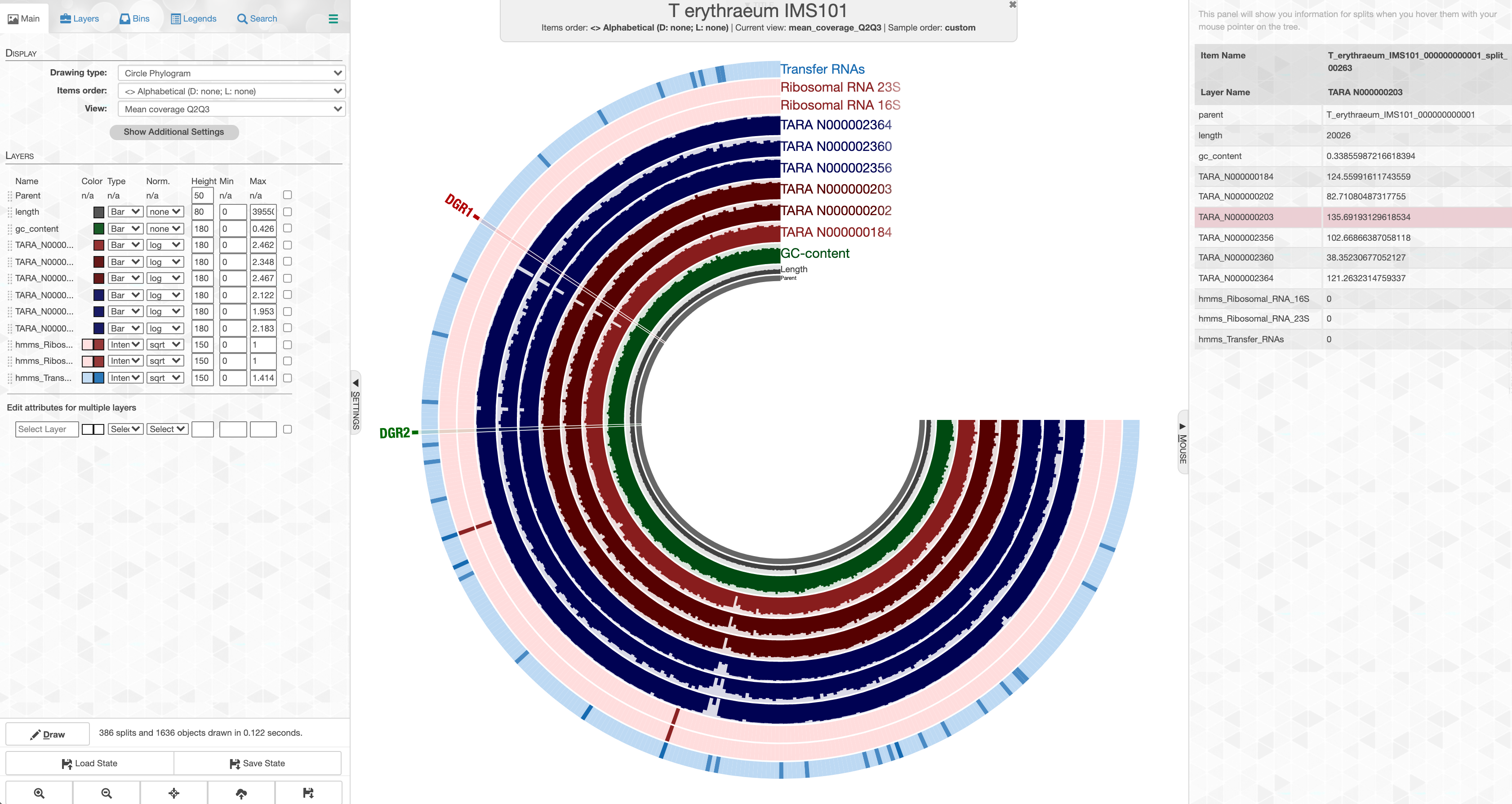
This is an anvi’o interactive interface, which provides a useful environment to explore read recruitment results. You can right-click on any item on shown on this page, and inspect the coverage of the genome across different metagenomes:
Even blindly go through a few sections of the genome to explore how the coverage looks like (which is something not many people does) is a useful exercise and will make you start wondering about how to make sense of weird things you see. Most bioinformatics approaches summarize coverage values per contig into a single number, even though there is so much to learn from actually just looking at them, so please feel free to take a moment to appreciate the sheer complexity of environmental metagenomes.
Looking for RTs in the genome
Exploring coverage patterns can certainly help life scientists who know their organisms to recognize interesting phenomena, but at some point one would like to focus on the task at hand, which, in the context of our study, was to find smoking guns of hypervariability.
In the case of DGRs, we know it is a good idea to start with retron-type reverse transcriptase genes. And when we have a contigs-db, searching for genes with particular functions, and highlighting the regions of the genome that contains genes with these functions can offer a good starting point to go deeper:

The same can also be done via the command line using the program anvi-search-functions.
Not all hits to the term “retron-type reverse transcriptase” will identify a gene that is a true RT, but browsing these small number of regions can help identify the true ones.
For instance, we found two regions that contained true RTs, and focused on one of these, which we denoted as DGR2 throughout our review. In the GIF above, it is one of those regions highlighted as red, which corresponds to T_erythraeum_IMS101_000000000001_split_00132 in our anvi’o databases. When there is a particular region of interest, you can find it on the interface by searching for this name to right-click and inspect it, or you can use the program anvi-inspect to visualize it. For instance, once you know which region you are interested in, running the following command in your terminal on our project files,
anvi-inspect -p PROFILE.db \
             -c CONTIGS.db \
             --split-name T_erythraeum_IMS101_000000000001_split_00132
will give you the following display with the RT:
The region shown in Panel B of our Figure 3 is around relative nucleotide positions of 8300 and 13500, and if you zoom into that region,
You will see the same region shown in Panel B. For trained eyes that have been looking at coverage data for a long time, the evidence for a DGR activity in this region is right there in this visualization. But let’s first take a look at this diagram that marks with tiny red boxes the locations of the template sequence the TR uses as well as the two DGR target sites in two genes:
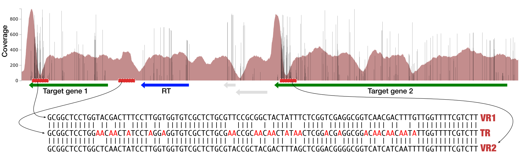
The alignment of sequences show that this is a text-book definition of DGR activity: sequences in both target sites differ from the template region (TR) only at adenosine nucleotides.
In fact, it is possible to confirm it visually. First, copy the entire sequence that matches to this region from the interface,
to search in a text editor the TR, which is this:
GCGGCTCCTGGAACAACTATCCTAGGAGGTGTCGCTCTGCGAACCGCAACAACTATAACTCGGACGAGGCGGACAACAACAATATTGGTTTTCGTCTT
but since we are working with the reverse-complemented genes (see the direction of the RT), we should search for the reverse complement of the template, which is this:
AAGACGAAAACCAATATTGTTGTTGTCCGCCTCGTCCGAGTTATAGTTGTTGCGGTTCGCAGAGCGACACCTCCTAGGATAGTTGTTCCAGGAGCCGC
There will be a single match, which will be the TR region, obviously:

But if we replace every T (instead of an A since the TR is reverse-complemented) with an N,
AAGACGAAAACCAA.A..G..G..G.CCGCC.CG.CCGAG..A.AG..G..GCGG..CGCAGAGCGACACC.CC.AGGA.AG..G..CCAGGAGCCGC
and search for this pattern instead, there will be multiple hits:
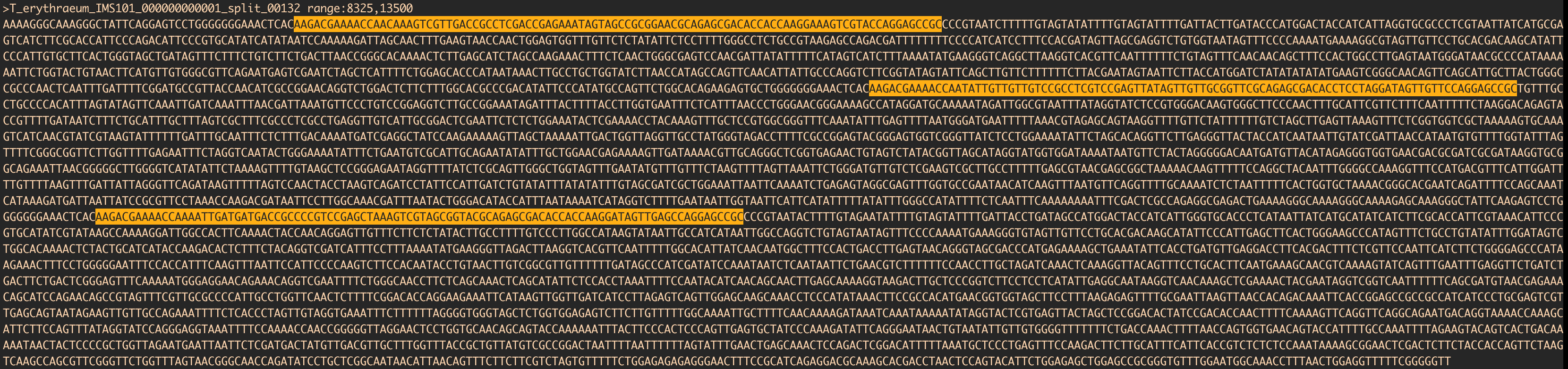
Poetic!
Visualizing coverage and single-nucleotide variants (SNVs)
So far we have been focusing on the genome, which essentially captures the state of the DGR-mediated evolution of the VRs at the time of sequencing of it. But of course what is even more interesting is to look into what has been happening in the environment.
For the sake of simplicity, from this point on we will focus only one of the VR regions:
To be specific, this region corresponds to this sequence:
>T_erythraeum_IMS101_000000000001_split_00132 range:8350,8827
TCCTGGGGGGGAAACTCACAAGACGAAAACCAACAAAGTCGTTGACCGCCTCGACCGAGAAATAGTAGCCGCGGAACGCAGAGCGACACCACCAAGGAAAGTCGTACCAGGAGCCGCCCC
GTAATCTTTTTGTAGTATATTTTGTAGTATTTTGATTACTTGATACCCATGGACTACCATCATTAGGTGCGCCCTCGTAATTATCATGCGAGTCATCTTCGCACCATTCCCAGACATTCC
CGTGCATATCATATAATCCAAAAAGATTAGCAACTTTGAAGTAACCAACTGGAGTGGTTTGTTCTCTATATTCTCCTTTTGGGCCTCTGCCGTAAGAGCCAGACGATTTTTTTTCCCCAT
CATCCTTTCCACGATAGTTAGCGAGGTCTGTGGTAATAGTTTCCCCAAAATGAAAAGGCGTAGTTGTTCCTGCACGACAAGCATATTCCCATTGTGCTTCACTGGGTAGCTGATAGT
Black bars indicate the positions of nucleotides in the genome that disagrees with the otherwise-homologous sequences found in the environment.
As we go into the variable region, the ‘mappability’ of reads start to decrease due to rapid increase in variation. This is an extremely straightforward way to recognize hypervariability that has emerged within the environmental populations. In addition to targeted analysis like this one (i.e., finding the RT, looking at upstream and downstream with expected outcomes), random walks throughout contigs may reveal new regions of potential interest.
Working with single-amino acid variants (SAAVs)
Variation in coverage and SNVs are quite effective indicators of within-population hypervariability in read recruitment results, however, SNVs are not sufficient indicators of change that influence amino acid composition. To address this we developed an algorithm to identify single-amino acid variants, or SAAVs, which we had first described in Delmont and Kiefl et al (2019)).
Sadly, while anvi’o displays SNVs in the interactive interface, it does not display SAAVs. But we clearly managed to show SAAVs in our figure instead of SNVs, anyway. How?
Anvi’o comes with one of the most powerful frameworks to study microbial population genetics (more info here), and enables extensive characterization of not only SNVs, but also single-codon variants (SCVs), as well as SAAVs. For instance, recovering SNVs, SCVs, or SAAVs of a gene, contig, or an entire genome in one or more metagenomes is possible via the program anvi-gen-variability-profile.
Since we know our gene of interest, we can instruct the program to focus only on it after learning the gene caller id of the gene of interest from the interface:
After this, we can run anvi-gen-variability-profile the following way,
anvi-gen-variability-profile -c CONTIGS.db \
                             -p PROFILE.db \
                             --gene-caller-ids 1687 \
                             --samples-of-interest samples-of-interest.txt \
                             -o DGR2_1687_AA.txt \
                             --engine AA \
                             --kiefl-mode
The samples-of-interest.txt is simply a text file that contains a single line that says TARA_N000000184, since in this figure we only used one of the six metagenomes as an example.
which would yield an output file that looks like this:
| entry_id | unique_pos_identifier | sample_id | corresponding_gene_call | codon_order_in_gene | codon_number | gene_length | coverage | Ala | Arg | Asn | Asp | Cys | Gln | Glu | Gly | His | Ile | Leu | Lys | Met | Phe | Pro | STP | Ser | Thr | Trp | Tyr | Val | reference | consensus | competing_aas | departure_from_reference | departure_from_consensus | n2n1ratio | entropy | BLOSUM90 | BLOSUM90_weighted | BLOSUM62 | BLOSUM62_weighted |
|---|---|---|---|---|---|---|---|---|---|---|---|---|---|---|---|---|---|---|---|---|---|---|---|---|---|---|---|---|---|---|---|---|---|---|---|---|---|---|---|
| (…) | (…) | (…) | (…) | (…) | (…) | (…) | (…) | (…) | (…) | (…) | (…) | (…) | (…) | (…) | (…) | (…) | (…) | (…) | (…) | (…) | (…) | (…) | (…) | (…) | (…) | (…) | (…) | (…) | (…) | (…) | (…) | (…) | (…) | (…) | (…) | (…) | (…) | (…) | (…) |
| 272 | 272 | TARA_N000000184 | 1687 | 246 | 247 | 879 | 1 | 0 | 0 | 0 | 0 | 0 | 0 | 0 | 0 | 0 | 0 | 0 | 1 | 0 | 0 | 0 | 0 | 0 | 0 | 0 | 0 | 0 | Lys | Lys | LysLys | 0.0 | 0.0 | 0.0 | 0.0 | 6.0 | 5.0 | ||
| 48 | 48 | TARA_N000000184 | 1687 | 247 | 248 | 879 | 139 | 2 | 0 | 0 | 0 | 0 | 0 | 0 | 0 | 0 | 16 | 0 | 0 | 0 | 0 | 0 | 0 | 0 | 0 | 0 | 0 | 121 | Arg | Val | IleVal | 1.0 | 0.12949640287769784 | 0.1322314049586777 | 0.43060076813672 | 3.0 | 2.489592760180997 | 3.0 | 2.6135746606334855 |
| 49 | 49 | TARA_N000000184 | 1687 | 248 | 249 | 879 | 133 | 0 | 0 | 0 | 0 | 0 | 0 | 0 | 0 | 0 | 0 | 121 | 0 | 0 | 0 | 0 | 0 | 5 | 0 | 0 | 0 | 7 | Leu | Leu | LeuVal | 0.09022556390977443 | 0.09022556390977443 | 0.05785123966942149 | 0.3643399806821796 | 0.0 | -1.2676529926025555 | 1.0 | -0.29119031607262946 |
| 273 | 273 | TARA_N000000184 | 1687 | 249 | 250 | 879 | 1 | 0 | 1 | 0 | 0 | 0 | 0 | 0 | 0 | 0 | 0 | 0 | 0 | 0 | 0 | 0 | 0 | 0 | 0 | 0 | 0 | 0 | Arg | Arg | ArgArg | 0.0 | 0.0 | 0.0 | 0.0 | 6.0 | 5.0 | ||
| 50 | 50 | TARA_N000000184 | 1687 | 250 | 251 | 879 | 108 | 0 | 0 | 0 | 0 | 0 | 0 | 0 | 105 | 0 | 0 | 0 | 0 | 0 | 0 | 0 | 1 | 2 | 0 | 0 | 0 | 0 | Gly | Gly | GlySer | 0.02777777777777779 | 0.027777777777777776 | 0.01904761904761905 | 0.1446114944607026 | -1.0 | -1.0000000000000013 | 0.0 | 0.0 |
| 274 | 274 | TARA_N000000184 | 1687 | 251 | 252 | 879 | 1 | 0 | 0 | 0 | 0 | 0 | 0 | 0 | 1 | 0 | 0 | 0 | 0 | 0 | 0 | 0 | 0 | 0 | 0 | 0 | 0 | 0 | Gly | Gly | GlyGly | 0.0 | 0.0 | 0.0 | 0.0 | 6.0 | 6.0 | ||
| 275 | 275 | TARA_N000000184 | 1687 | 252 | 253 | 879 | 1 | 0 | 0 | 0 | 0 | 0 | 0 | 0 | 0 | 0 | 0 | 0 | 0 | 0 | 0 | 0 | 0 | 1 | 0 | 0 | 0 | 0 | Ser | Ser | SerSer | 0.0 | 0.0 | 0.0 | 0.0 | 5.0 | 4.0 | ||
| 276 | 276 | TARA_N000000184 | 1687 | 253 | 254 | 879 | 1 | 0 | 0 | 0 | 0 | 0 | 0 | 0 | 0 | 0 | 0 | 0 | 0 | 0 | 0 | 0 | 0 | 0 | 0 | 1 | 0 | 0 | Trp | Trp | TrpTrp | 0.0 | 0.0 | 0.0 | 0.0 | 11.0 | 11.0 | ||
| 51 | 51 | TARA_N000000184 | 1687 | 254 | 255 | 879 | 67 | 0 | 0 | 5 | 4 | 1 | 0 | 0 | 0 | 0 | 1 | 5 | 0 | 0 | 22 | 0 | 0 | 1 | 0 | 0 | 28 | 0 | Tyr | Tyr | PheTyr | 0.582089552238806 | 0.582089552238806 | 0.7857142857142857 | 1.4741819204714253 | 3.0 | -0.5564720812182741 | 3.0 | 0.048857868020304465 |
| 52 | 52 | TARA_N000000184 | 1687 | 255 | 256 | 879 | 63 | 0 | 0 | 12 | 8 | 0 | 0 | 0 | 0 | 0 | 0 | 1 | 0 | 0 | 16 | 0 | 0 | 2 | 0 | 0 | 17 | 7 | Asp | Tyr | PheTyr | 0.873015873015873 | 0.7301587301587301 | 0.9411764705882353 | 1.6988787908328986 | 3.0 | -2.0360531309297913 | 3.0 | -1.0961416824794434 |
| 53 | 53 | TARA_N000000184 | 1687 | 256 | 257 | 879 | 68 | 0 | 0 | 5 | 1 | 3 | 0 | 0 | 2 | 0 | 6 | 4 | 0 | 0 | 19 | 0 | 0 | 2 | 0 | 0 | 25 | 1 | Phe | Tyr | PheTyr | 0.7205882352941176 | 0.6323529411764706 | 0.76 | 1.7661608575859613 | 3.0 | -1.1439864483342745 | 3.0 | -0.3387916431394694 |
| 277 | 277 | TARA_N000000184 | 1687 | 257 | 258 | 879 | 1 | 0 | 0 | 0 | 0 | 0 | 0 | 0 | 0 | 0 | 0 | 0 | 0 | 0 | 0 | 1 | 0 | 0 | 0 | 0 | 0 | 0 | Pro | Pro | ProPro | 0.0 | 0.0 | 0.0 | 0.0 | 8.0 | 7.0 | ||
| 54 | 54 | TARA_N000000184 | 1687 | 258 | 259 | 879 | 77 | 0 | 36 | 0 | 0 | 0 | 0 | 0 | 14 | 0 | 0 | 0 | 0 | 0 | 0 | 0 | 0 | 0 | 0 | 27 | 0 | 0 | Trp | Arg | ArgTrp | 0.6493506493506493 | 0.5324675324675324 | 0.75 | 1.0328823078127687 | -4.0 | -3.7281553398058254 | -3.0 | -2.5242718446601944 |
| 55 | 55 | TARA_N000000184 | 1687 | 259 | 260 | 879 | 84 | 0 | 18 | 0 | 0 | 0 | 0 | 0 | 3 | 0 | 0 | 0 | 0 | 0 | 0 | 0 | 0 | 0 | 0 | 63 | 0 | 0 | Trp | Trp | ArgTrp | 0.25 | 0.25 | 0.2857142857142857 | 0.6648642241909106 | -4.0 | -3.96078431372549 | -3.0 | -2.823529411764706 |
| 278 | 278 | TARA_N000000184 | 1687 | 260 | 261 | 879 | 1 | 0 | 0 | 0 | 0 | 1 | 0 | 0 | 0 | 0 | 0 | 0 | 0 | 0 | 0 | 0 | 0 | 0 | 0 | 0 | 0 | 0 | Cys | Cys | CysCys | 0.0 | 0.0 | 0.0 | 0.0 | 9.0 | 9.0 | ||
| 279 | 279 | TARA_N000000184 | 1687 | 261 | 262 | 879 | 1 | 0 | 1 | 0 | 0 | 0 | 0 | 0 | 0 | 0 | 0 | 0 | 0 | 0 | 0 | 0 | 0 | 0 | 0 | 0 | 0 | 0 | Arg | Arg | ArgArg | 0.0 | 0.0 | 0.0 | 0.0 | 6.0 | 5.0 | ||
| 280 | 280 | TARA_N000000184 | 1687 | 262 | 263 | 879 | 1 | 0 | 0 | 0 | 0 | 0 | 0 | 0 | 0 | 0 | 0 | 0 | 0 | 0 | 0 | 0 | 0 | 1 | 0 | 0 | 0 | 0 | Ser | Ser | SerSer | 0.0 | 0.0 | 0.0 | 0.0 | 5.0 | 4.0 | ||
| 281 | 281 | TARA_N000000184 | 1687 | 263 | 264 | 879 | 1 | 1 | 0 | 0 | 0 | 0 | 0 | 0 | 0 | 0 | 0 | 0 | 0 | 0 | 0 | 0 | 0 | 0 | 0 | 0 | 0 | 0 | Ala | Ala | AlaAla | 0.0 | 0.0 | 0.0 | 0.0 | 5.0 | 4.0 | ||
| 56 | 56 | TARA_N000000184 | 1687 | 264 | 265 | 879 | 149 | 0 | 0 | 13 | 14 | 1 | 0 | 0 | 1 | 0 | 13 | 18 | 0 | 0 | 39 | 0 | 0 | 3 | 0 | 0 | 42 | 5 | Phe | Tyr | PheTyr | 0.738255033557047 | 0.7181208053691275 | 0.9285714285714286 | 1.870615888859036 | 3.0 | -1.5474420153146153 | 3.0 | -0.7085784041726777 |
| 282 | 282 | TARA_N000000184 | 1687 | 265 | 266 | 879 | 1 | 0 | 1 | 0 | 0 | 0 | 0 | 0 | 0 | 0 | 0 | 0 | 0 | 0 | 0 | 0 | 0 | 0 | 0 | 0 | 0 | 0 | Arg | Arg | ArgArg | 0.0 | 0.0 | 0.0 | 0.0 | 6.0 | 5.0 | ||
| 57 | 57 | TARA_N000000184 | 1687 | 266 | 267 | 879 | 183 | 0 | 2 | 27 | 39 | 0 | 0 | 0 | 16 | 1 | 6 | 22 | 0 | 0 | 21 | 0 | 0 | 20 | 0 | 0 | 23 | 6 | Gly | Asp | AsnAsp | 0.912568306010929 | 0.7868852459016393 | 0.6923076923076923 | 2.1325230668720696 | 1.0 | -2.4990362109321214 | 1.0 | -1.497865895635412 |
| 58 | 58 | TARA_N000000184 | 1687 | 267 | 268 | 879 | 231 | 0 | 7 | 58 | 11 | 2 | 0 | 0 | 5 | 0 | 15 | 20 | 0 | 0 | 28 | 0 | 0 | 11 | 0 | 0 | 58 | 16 | Tyr | Asn | AsnTyr | 0.748917748917749 | 0.7489177489177489 | 1.0 | 2.044069292686376 | -3.0 | -2.2779967747715464 | -2.0 | -1.3312130442573014 |
| 59 | 59 | TARA_N000000184 | 1687 | 268 | 269 | 879 | 253 | 0 | 0 | 0 | 1 | 10 | 0 | 0 | 0 | 0 | 0 | 0 | 0 | 0 | 29 | 0 | 0 | 18 | 0 | 1 | 194 | 0 | Tyr | Tyr | PheTyr | 0.23320158102766797 | 0.233201581027668 | 0.14948453608247422 | 0.8113791942612562 | 3.0 | -0.38819405719748273 | 3.0 | 0.3066995937226163 |
| 60 | 60 | TARA_N000000184 | 1687 | 269 | 270 | 879 | 287 | 2 | 0 | 11 | 4 | 1 | 0 | 0 | 1 | 2 | 26 | 46 | 0 | 0 | 84 | 0 | 0 | 7 | 0 | 0 | 79 | 24 | Phe | Phe | PheTyr | 0.7073170731707317 | 0.7073170731707317 | 0.9404761904761905 | 1.8170003941079511 | 3.0 | -0.7784392745924161 | 3.0 | -0.04326189167735232 |
| 61 | 61 | TARA_N000000184 | 1687 | 270 | 271 | 879 | 326 | 0 | 0 | 0 | 0 | 0 | 0 | 0 | 0 | 0 | 0 | 4 | 0 | 0 | 3 | 1 | 0 | 318 | 0 | 0 | 0 | 0 | Ser | Ser | LeuSer | 0.024539877300613466 | 0.024539877300613498 | 0.012578616352201259 | 0.1391263567207563 | -3.0 | -2.864611783066717 | -2.0 | -1.870464299648848 |
| 62 | 62 | TARA_N000000184 | 1687 | 271 | 272 | 879 | 372 | 5 | 0 | 2 | 57 | 0 | 0 | 0 | 16 | 0 | 2 | 4 | 0 | 0 | 3 | 0 | 0 | 0 | 0 | 0 | 0 | 283 | Val | Val | AspVal | 0.239247311827957 | 0.239247311827957 | 0.20141342756183744 | 0.8325024390840705 | -5.0 | -4.1310750566396255 | -3.0 | -2.392567419425565 |
| 63 | 63 | TARA_N000000184 | 1687 | 272 | 273 | 879 | 416 | 1 | 0 | 0 | 1 | 0 | 1 | 368 | 9 | 1 | 0 | 0 | 2 | 1 | 0 | 0 | 0 | 0 | 0 | 0 | 0 | 32 | Glu | Glu | GluVal | 0.11538461538461542 | 0.11538461538461539 | 0.08695652173913043 | 0.4868405831148602 | -3.0 | -2.640725121857714 | -2.0 | -1.6656991072895562 |
| 64 | 64 | TARA_N000000184 | 1687 | 273 | 274 | 879 | 444 | 163 | 0 | 0 | 1 | 0 | 0 | 1 | 1 | 0 | 0 | 3 | 1 | 11 | 0 | 2 | 0 | 67 | 186 | 1 | 0 | 7 | Ala | Thr | AlaThr | 0.6328828828828829 | 0.581081081081081 | 0.8763440860215054 | 1.3015342024938332 | 0.0 | 0.06597407345347082 | 0.0 | 0.19405304126616596 |
| 65 | 65 | TARA_N000000184 | 1687 | 274 | 275 | 879 | 464 | 9 | 0 | 6 | 178 | 0 | 0 | 3 | 46 | 0 | 0 | 2 | 0 | 0 | 11 | 0 | 0 | 0 | 3 | 0 | 1 | 205 | Val | Val | AspVal | 0.5581896551724138 | 0.5581896551724138 | 0.8682926829268293 | 1.2808922763228758 | -5.0 | -4.0563896271819555 | -3.0 | -2.380892177286114 |
| 66 | 66 | TARA_N000000184 | 1687 | 275 | 276 | 879 | 513 | 0 | 8 | 167 | 88 | 0 | 0 | 2 | 10 | 8 | 41 | 22 | 1 | 0 | 26 | 0 | 0 | 47 | 10 | 0 | 69 | 14 | Asn | Asn | AsnAsp | 0.6744639376218324 | 0.6744639376218323 | 0.5269461077844312 | 2.0600679413792027 | 1.0 | -2.0710786570655073 | 1.0 | -1.1917346544135248 |
| 67 | 67 | TARA_N000000184 | 1687 | 276 | 277 | 879 | 546 | 1 | 0 | 157 | 174 | 0 | 0 | 0 | 13 | 2 | 13 | 23 | 0 | 0 | 20 | 2 | 0 | 39 | 2 | 1 | 73 | 26 | Asp | Asp | AsnAsp | 0.6813186813186813 | 0.6813186813186813 | 0.9022988505747126 | 1.8425864744458764 | 1.0 | -2.028227182742849 | 1.0 | -1.1755409925592188 |
| 68 | 68 | TARA_N000000184 | 1687 | 277 | 278 | 879 | 591 | 12 | 10 | 81 | 66 | 4 | 0 | 0 | 9 | 3 | 65 | 61 | 0 | 0 | 113 | 3 | 0 | 31 | 7 | 0 | 87 | 39 | Phe | Phe | PheTyr | 0.8087986463620982 | 0.8087986463620981 | 0.7699115044247787 | 2.278592016934293 | 3.0 | -2.1815553891728245 | 3.0 | -1.244265763859501 |
| 69 | 69 | TARA_N000000184 | 1687 | 278 | 279 | 879 | 671 | 0 | 0 | 0 | 0 | 0 | 0 | 0 | 0 | 0 | 445 | 17 | 0 | 14 | 137 | 0 | 0 | 0 | 0 | 0 | 0 | 58 | Val | Ile | IlePhe | 0.9135618479880775 | 0.33681073025335323 | 0.30786516853932583 | 0.9822451928916645 | -1.0 | 0.11259679962369017 | 0.0 | 0.8111394698560093 |
| 283 | 283 | TARA_N000000184 | 1687 | 279 | 280 | 879 | 1 | 0 | 0 | 0 | 0 | 0 | 0 | 0 | 1 | 0 | 0 | 0 | 0 | 0 | 0 | 0 | 0 | 0 | 0 | 0 | 0 | 0 | Gly | Gly | GlyGly | 0.0 | 0.0 | 0.0 | 0.0 | 6.0 | 6.0 | ||
| 284 | 284 | TARA_N000000184 | 1687 | 280 | 281 | 879 | 1 | 0 | 0 | 0 | 0 | 0 | 0 | 0 | 0 | 0 | 0 | 0 | 0 | 0 | 1 | 0 | 0 | 0 | 0 | 0 | 0 | 0 | Phe | Phe | PhePhe | 0.0 | 0.0 | 0.0 | 0.0 | 7.0 | 6.0 | ||
| 285 | 285 | TARA_N000000184 | 1687 | 281 | 282 | 879 | 1 | 0 | 1 | 0 | 0 | 0 | 0 | 0 | 0 | 0 | 0 | 0 | 0 | 0 | 0 | 0 | 0 | 0 | 0 | 0 | 0 | 0 | Arg | Arg | ArgArg | 0.0 | 0.0 | 0.0 | 0.0 | 6.0 | 5.0 | ||
| 286 | 286 | TARA_N000000184 | 1687 | 282 | 283 | 879 | 1 | 0 | 0 | 0 | 0 | 0 | 0 | 0 | 0 | 0 | 0 | 1 | 0 | 0 | 0 | 0 | 0 | 0 | 0 | 0 | 0 | 0 | Leu | Leu | LeuLeu | 0.0 | 0.0 | 0.0 | 0.0 | 5.0 | 4.0 | ||
| 287 | 287 | TARA_N000000184 | 1687 | 283 | 284 | 879 | 1 | 0 | 0 | 0 | 0 | 0 | 0 | 0 | 0 | 0 | 0 | 0 | 0 | 0 | 0 | 0 | 0 | 0 | 0 | 0 | 0 | 1 | Val | Val | ValVal | 0.0 | 0.0 | 0.0 | 0.0 | 5.0 | 4.0 | ||
| 288 | 288 | TARA_N000000184 | 1687 | 284 | 285 | 879 | 1 | 0 | 0 | 0 | 0 | 0 | 0 | 0 | 0 | 0 | 0 | 0 | 0 | 0 | 0 | 0 | 0 | 1 | 0 | 0 | 0 | 0 | Ser | Ser | SerSer | 0.0 | 0.0 | 0.0 | 0.0 | 5.0 | 4.0 | ||
| 70 | 70 | TARA_N000000184 | 1687 | 285 | 286 | 879 | 902 | 0 | 0 | 0 | 0 | 0 | 0 | 0 | 0 | 0 | 3 | 0 | 0 | 0 | 797 | 0 | 0 | 2 | 0 | 0 | 0 | 100 | Phe | Phe | PheVal | 0.11640798226164084 | 0.1164079822616408 | 0.12547051442910917 | 0.38572280296535677 | -2.0 | -1.972788065232625 | -1.0 | -0.9787269423097479 |
| 289 | 289 | TARA_N000000184 | 1687 | 286 | 287 | 879 | 1 | 0 | 0 | 0 | 0 | 0 | 0 | 0 | 0 | 0 | 0 | 0 | 0 | 0 | 0 | 1 | 0 | 0 | 0 | 0 | 0 | 0 | Pro | Pro | ProPro | 0.0 | 0.0 | 0.0 | 0.0 | 8.0 | 7.0 | ||
| 290 | 290 | TARA_N000000184 | 1687 | 287 | 288 | 879 | 1 | 0 | 0 | 0 | 0 | 0 | 0 | 0 | 0 | 0 | 0 | 0 | 0 | 0 | 0 | 1 | 0 | 0 | 0 | 0 | 0 | 0 | Pro | Pro | ProPro | 0.0 | 0.0 | 0.0 | 0.0 | 8.0 | 7.0 | ||
| 291 | 291 | TARA_N000000184 | 1687 | 288 | 289 | 879 | 1 | 0 | 1 | 0 | 0 | 0 | 0 | 0 | 0 | 0 | 0 | 0 | 0 | 0 | 0 | 0 | 0 | 0 | 0 | 0 | 0 | 0 | Arg | Arg | ArgArg | 0.0 | 0.0 | 0.0 | 0.0 | 6.0 | 5.0 | ||
| 71 | 71 | TARA_N000000184 | 1687 | 289 | 290 | 879 | 923 | 116 | 0 | 0 | 0 | 0 | 0 | 0 | 0 | 0 | 0 | 0 | 0 | 0 | 0 | 4 | 0 | 0 | 803 | 0 | 0 | 0 | Thr | Thr | AlaThr | 0.1300108342361863 | 0.13001083423618634 | 0.1444582814445828 | 0.40540770155369993 | 0.0 | -0.07113938692886063 | 0.0 | -0.03796579360489136 |
| 72 | 72 | TARA_N000000184 | 1687 | 290 | 291 | 879 | 923 | 0 | 0 | 0 | 0 | 0 | 0 | 0 | 0 | 0 | 0 | 351 | 0 | 0 | 32 | 509 | 0 | 28 | 3 | 0 | 0 | 0 | Pro | Pro | LeuPro | 0.44853737811484296 | 0.4485373781148429 | 0.6895874263261297 | 0.9371058142414911 | -4.0 | -3.6159630635059727 | -3.0 | -2.7339717418720464 |
| 73 | 73 | TARA_N000000184 | 1687 | 291 | 292 | 879 | 915 | 0 | 0 | 0 | 1 | 0 | 31 | 860 | 0 | 0 | 0 | 0 | 20 | 0 | 0 | 0 | 3 | 0 | 0 | 0 | 0 | 0 | Glu | Glu | GlnGlu | 0.060109289617486295 | 0.060109289617486336 | 0.03604651162790698 | 0.28272085169189326 | 2.0 | 1.2061642175761718 | 2.0 | 1.6047234033178384 |
| 292 | 292 | TARA_N000000184 | 1687 | 292 | 293 | 879 | 1 | 0 | 0 | 0 | 0 | 0 | 0 | 0 | 0 | 0 | 0 | 0 | 0 | 0 | 0 | 0 | 1 | 0 | 0 | 0 | 0 | 0 | STP | STP | STPSTP | 0.0 | 0.0 | 0.0 | 0.0 |
This file (which scrolls to the right quite a bit), shows for each codon position in this gene, the variability of environmental sequences. The power of this approach comes from the fact that SAAVs represent the allele frequency of amino acids in a single codon position based on the number of short reads that fully cover the codon (which is described here). That’s why the matrix in this output file where the frequencies of individual amino acids are shown is full of zeros for most positions that are outside the VR, yet there clearly is a tremendous amount of amino acid diversity in the environment within the VR site!
Visualizing this information is indeed a challenge, but thanks to the comprehensive output file anvi’o generates, it is not impossible with a few lines of R code. Here is what I wrote for this:
#!/usr/bin/env Rscript
library(ggplot2)
library(reshape2)
library(reshape)
require(gridExtra)

# a color palette to use for amino acids later. it is slightly
# modified by Kevin Wright's beautiful template here:
# https://stackoverflow.com/a/9568659
c25 <- c("dodgerblue2", "#E31A1C", "green4", "#6A3D9A",
         "#FF7F00", "yellow4", "gold1", "skyblue2", "#FB9A99",
         "palegreen2", "#CAB2D6", "#FDBF6F", "gray70", "brown",
         "maroon", "orchid1", "deeppink1", "blue1", "steelblue4",
         "darkturquoise", "darkorange4", "white")

# boring theme thingies
F <- theme(panel.border = element_blank(),
           plot.margin = unit(c(0.6,0.3,1,0.3), "cm"),
           axis.title.y=element_blank(),
           axis.title.x=element_blank(),
           axis.line.x = element_blank(),
           axis.text.x = element_text(face = "bold"),
           axis.text.y = element_text(face = "bold"),
           panel.grid.major = element_blank(),
           panel.grid.minor = element_blank(),
           axis.line.y = element_blank(),
           axis.ticks.x = element_blank(),
           axis.ticks.y = element_blank(),
           plot.title = element_text(color = "#222222", size = 14, face = "bold"),
           plot.subtitle = element_text(color = "#444444", size = 10))

# read in the data, which is the output of anvi-gen-variabiliyt-profile
df <- read.table(file='DGR2_1687_AA.txt', header = TRUE, sep = "\t")

# focus on on the codons that are closer to the VR
df <- df[df$codon_order_in_gene > 125, ]

# get dx from df, a simplified data frame that only contains codon order
# and amino acid frequencies, so we can melt it into a sweet, long-format
# dataframe that is easier to visualize with ggplot:
columns_to_keep <- c("codon_order_in_gene", "Ala", "Arg", "Asn", "Asp", "Cys",
                     "Gln", "Glu", "Gly", "His", "Ile", "Leu", "Lys", "Met",
                     "Phe", "Pro", "STP", "Ser", "Thr", "Trp", "Tyr", "Val")
dx <- melt(df[, (names(df) %in% columns_to_keep)], id="codon_order_in_gene")
names(dx) <- c("codon", "aa", "freq")
dx$aa <- as.character(dx$aa)

# we will learn the dominant amino acid per codon position, and name it
# `ZREF` so we can set an ugly color to only focus on variable sites
for (codon_num in unique(dx$codon)){
  dxm <- dx[dx$codon == codon_num, ]
  dominant_aa <- as.character(tail(dxm[order(dxm$freq), ], n=1)$aa)
  dx[dx$codon == codon_num & dx$aa == dominant_aa, "aa"] <- 'ZREF'
}

# generate the plot object
p <- ggplot(dx, aes(x=codon, y=freq, fill=aa))
p <- p + geom_bar(position="fill", stat="identity")
p <- p + theme(legend.position="bottom")
p <- p + scale_fill_manual(values = c25)
p <- p + scale_y_reverse() + scale_x_reverse()
p <- p + ggtitle('Single amino acid variants')
p <- p + F

# print it into a PDF file!
pdf(file = "SAAVs.pdf",  width = 15, height = 5)
print(p)
dev.off()
Running this code generates this image in a PDF file,

which was straightforward to overlay on the coverage data to generate the following in our beloved Inkscape:
Some SNVs do not have a corresponding SAAV, since not every single-nucleotide variant is non-synonymous.
We are about to move on to an entirely different way to look at these data. But I would like to point out here as a reminder that the output file generated by the program anvi-gen-variability-profile can serve many purposes for much more in-depth analyses of evolution and microbial population genetics.
Defining an in silico primer and collecting reads
So far we investigated the coverage patterns in a region of a genome that is influenced by the activities of a retroelement, visualized single-nucleotide variants in that region, and confirmed the extensive amino acid diversification of the environmental populations of Trichodesmium erythraeum at this site. For all these investigations, we used a single metagenome for simplicity. But for those who are interested in microdiversity or hypervariability, the question sooner or later comes to those that are of ecology as we inevitably wonder whether these patterns conserved across environments or there is any evidence that they respond to environmental change.
In other words, can you squint your eyes looking at the figure below that shows all the SNVs in that most variable region of the DGR2 across all metagenomes, and tell if some metagenomes are more similar to one another than others** or if each metagenome seems to have a random collection of variants as if sequences were evolving on a Brownian motion path? And if there are groups of metagenomes in which DGR activity seems to create similar diversity patterns, can you tell whether biogeography explains the similarities and differences? Of course these are worthy questions to go after as our answers to them may have significant implications on our ability to ask better questions to understand the role of DGRs (or any other genetic mechanism that tinker with the speed of evolution) on the lifestyles of environmental microbes.
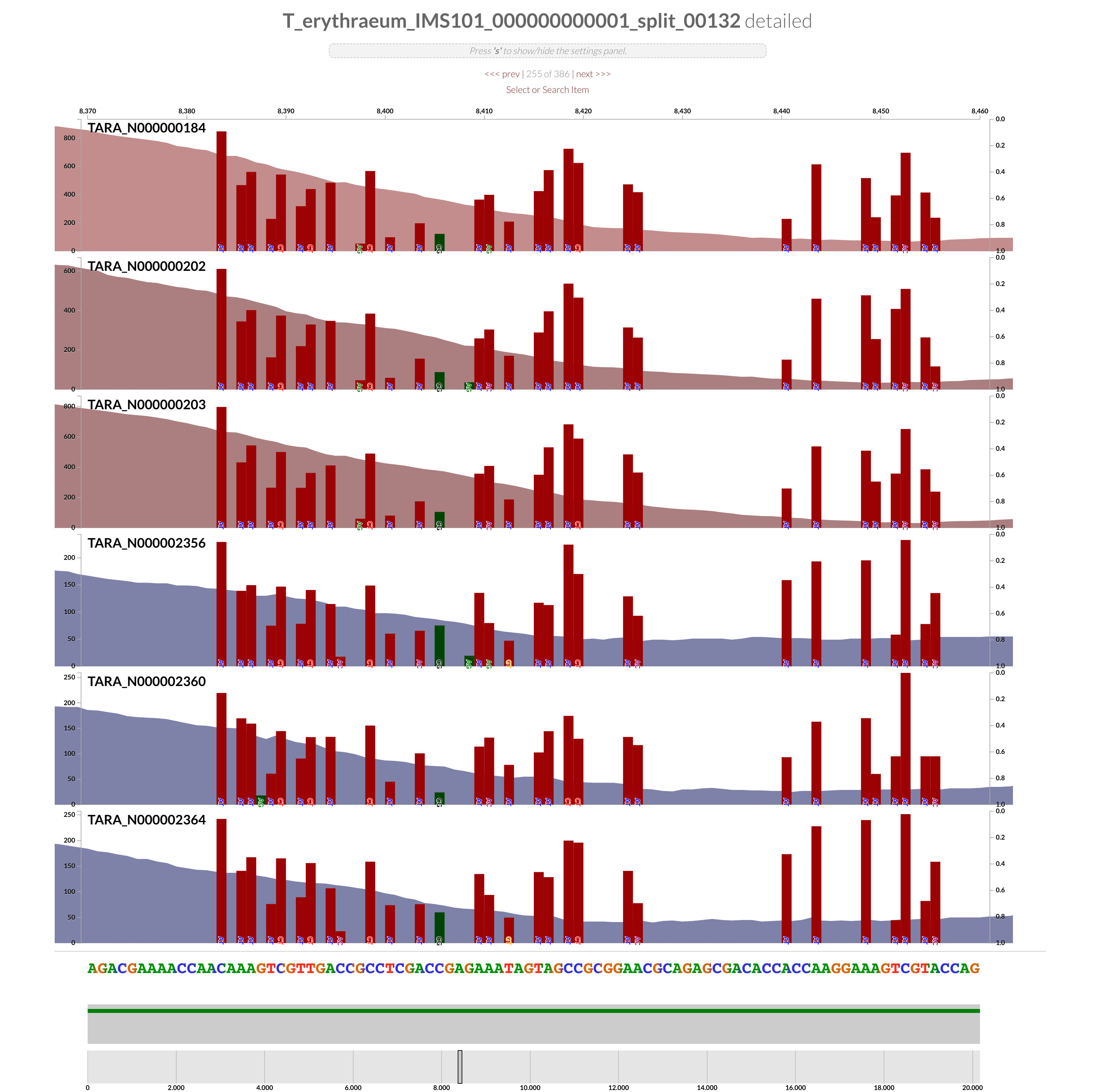
We will get back to whether you can squint your eyes or not to answer those important questions. But there is something that is worth noting here before moving on. The green bars for SNVs in the anvi’o inspection page mark SNVs that are at the third nucleotide position of a given codon, while red ones indicate those that occur at the first or the second nucleotide positions in codons. Changes in the first and second nucleotide positions in a codon are much more likely to influence the amino acid identity than those that occur in the third (since only 30% of changes at the third codon positions will result in a different amino acid). When you look at metagenomes and SNVs long enough, you realize that if you use a genome to recruit reads from a metagenome that contains very closely related populations. genomes of which are almost identical to your reference genome but not quite, most differences between them that yield SNVs occur in the third nucleotide positions of codons. Because, you know, evolution. And there is something magical in being able to see something so fundamental to DGRs even in this little figure above, as a software platform that is absolutely indifferent to DGRs is simply showing us how almost all variation in this region is in the first and second nucleotide positions of codons.
And going back to the topic, no, even though as a computer scientist I very much believe in the power of squinting eyes to understand biology, in some cases we just can’t use that strategy to find answers to some questions. In fact, when variability is so high, we can’t even trust reads that we were able to recruit: the sudden drop in coverage tells us clearly that there are many more reads in the environment that would have matched to this very region, but our mapping software could not place them here. Due to extreme variation, they were no longer have the minimum sequence identity to this reference to be recruited. Working with mapped reads is the field standard. But we clearly need to go back to the raw reads and recover those we are missing.
Luckily, the anvi’o program anvi-script-get-primer-matches does exactly that for us. It takes in a primers-txt, in which we describe a pattern we are interested in, and a samples-txt file, to find all the short reads that match to those patterns and report a FASTA file for each one of them. We already have our samples-txt that looks like this:
| sample | r1 | r2 |
|---|---|---|
| TARA_N000002360 | ERR1726621_1.fastq.gz | ERR1726621_2.fastq.gz |
| TARA_N000000202 | ERR1726854_1.fastq.gz | ERR1726854_2.fastq.gz |
| TARA_N000002356 | ERR1726640_1.fastq.gz,ERR1726924_1.fastq.gz | ERR1726640_2.fastq.gz,ERR1726924_2.fastq.gz |
| TARA_N000000184 | ERR1726697_1.fastq.gz | ERR1726697_2.fastq.gz |
| TARA_N000002364 | ERR1726823_1.fastq.gz | ERR1726823_2.fastq.gz |
| TARA_N000000203 | ERR1726921_1.fastq.gz | ERR1726921_2.fastq.gz |
The key part is to define the pattern that would bring us all the short reads that extend into the variable region. For this, we can combine what we learn from the genome and what we learn the environment through SNVs.
This is how our genome sequence looks like in that region (we know that since we zoom in enough, anvi’o shows us the nucleotides matching to each position):
Looking at this, one can design a primer sequence that demands all the nucleotides that is conserved to be present while embracing all the variation for the remaining nucleotide positions. The key is to make sure it is long enough to cover all the conserved regions, but not too long so its total length is not longer than the read length of the metagenomic sequences.
Here is one that takes all into consideration to recover as many metagenomic reads from FASTQ files with as much stringency as possible to understand the variation in this region by cutting off the middle-man, the enemy of hypervariability, the mapping software:
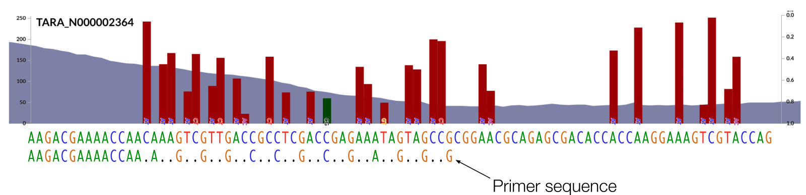
The program anvi-script-get-primer-matches uses ‘regular expressions’ (here is a cheat sheet) where . is equivalent to an N in primer design and means ‘any character is OK here’.
Another way to do it would have been to use the TR sequence and replace every T (not an A since it is reverse complemented) with a ., but doing it based on the environment is a more stringent way to do that. Although, it would certainly be a decision that should be made per question basis.
Now, we know our ‘primer’ sequence, and thus we can generate the primers-txt file:
| name | primer_sequence |
|---|---|
| DGR2_VR1 | AAGACGAAAACCAA.A..G..G..G..C..C..G..C..G..A..G..G..G |
Now running this will get all the matching reads from each metagenome:
anvi-script-get-primer-matches --primers-txt primers.txt \
                               --samples samples.txt \
                               --only-report-primer-match \
                               -o PRIMER-MATCHES
As explained in the program help menu, the flag --only-report-primer-match will only report the parts of sequences that match to the primer and will trim the rest.
When the program is done running, the output directory PRIMER-MATCHES will be populated by as many FASTA files as there are metagenomes x primers (which is 1 in our case), and will look like this:
ls PRIMER-MATCHES/

TARA_N000000184-DGR2_VR1-HITS.fa
TARA_N000000202-DGR2_VR1-HITS.fa
TARA_N000000203-DGR2_VR1-HITS.fa
TARA_N000002356-DGR2_VR1-HITS.fa
TARA_N000002360-DGR2_VR1-HITS.fa
TARA_N000002364-DGR2_VR1-HITS.fa
And each FASTA files will contain reads that are of equal length, and matching 100% to the primer we defined:
>TARA_N000002364_DGR2_VR1_00001
AAGACGAAAACCAATAACGCTGAAGTCCGCCTCGACCGAGTAAGAGTAGTAG
>TARA_N000002364_DGR2_VR1_00002
AAGACGAAAACCAATATCGTTGACGTCCGTCTCGACCGAGTAATAGAAGTTG
>TARA_N000002364_DGR2_VR1_00003
AAGACGAAAACCAATATTGTTGTTGTCCGTCTCGTCCGAGTTATAGTTGTTG
>TARA_N000002364_DGR2_VR1_00004
AAGACGAAAACCAAAATTGTTGTCGTCCGTCACGACCGAGTAATAGTTGAGG
>TARA_N000002364_DGR2_VR1_00005
AAGACGAAAACCAATATTGTTGTTGTCCGTCTCGTCCGAGTTATAGTTGTTG
>TARA_N000002364_DGR2_VR1_00006
AAGACGAAAACCAATATTGCCGCTGACCGCCTCGCCCGAGTAATAGAAGCAG
>TARA_N000002364_DGR2_VR1_00007
AAGACGAAAACCAATATTGTTGTTGTCCGTCTCGTCCGAGTTATAGTTGTTG
>TARA_N000002364_DGR2_VR1_00008
AAGACGAAAACCAACATGGCTGTAGTCCGACTCGCCCGAGTAATAGTCGAGG
>TARA_N000002364_DGR2_VR1_00009
AAGACGAAAACCAATAACGTCGCTGACCGTCTCGTCCGAGAAAGAGTAGTCG
>TARA_N000002364_DGR2_VR1_00010
AAGACGAAAACCAATAAAGTCGTAGTCCGACTCGACCGAGACATAGTAGTGG
(...)
Finally, one can put all the short reads into a single file so we can think about how to make sense of them:
cat PRIMER-MATCHES/*-DGR2_VR1-HITS.fa > DGR2-VR1-HITS.fa
Performing an oligotyping analysis
The FASTA file DGR2-VR1-HITS.fa contains all the sequences we need to think about the ecology of the DGR activity. Opening it in any program to study sequence alignments will already yield a lot of insights, but if our desire is to compare distinct environments based on their DGR profiles, we somehow need to divide sequences in this file into meaningful groups. At this stage using taxonomy for this is obviously out of question, since we are studying a single taxon. Another option could be using de novo sequence similarities, a problem you may be familiar with from amplicon sequencing, where 16S rRNA gene amplicons must be first turned into operational units based on arbitrary sequence similarity thresholds and compared across samples. We could do that, but the extremely high diversity within these sequences would either yield way too many OTUs with high similarity thresholds or too little OTUs with too much diversity within with low similarity thresholds. We could also use denoising algorithms such as DADA2, but our problem requires much more subtle access to diversity, rather than trying to tame it.
By focusing only on a user-defined number of high-entropy nucleotide positions to decompose a group of sequences, oligotyping offers a very good and scalable solution for this problem with room for extensive supervision. Even though it was designed for 16S rRNA gene amplicons, it has quite useful applications to metagenomics to study microdiversity and/or hypervariability.
Anvi’o already includes programs such as anvi-report-linkmers and anvi-oligotype-linkmers to resolve oligotypes through physically connected nucleotide positions, but since we already have our sequences of interest in a FASTA file, here we can use the stand-alone oligotyping pipeline (which is easy to install and run) to also get summary figures without any additional effort.
As per the instructions on how to run an oligotyping analysis on a given set of sequences, the first step is to calculate the entropy in the file, which we can do the following way on our FASTA file:
entropy-analysis DGR2-VR1-HITS.fa --quick
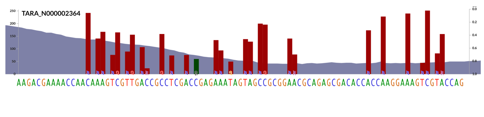
At the end of this analysis, oligotyping greets us with a figure that shows the entropy results:

Which are exactly as we would have expected given our primer. So far so good. The next step is to run the oligotyping analysis:
oligotype DGR2-VR1-HITS.fa \
          DGR2-VR1-HITS.fa-ENTROPY \
          --number-of-auto-components 10 \
          --min-substantive-abundance 8 \
          --output-directory DGR2-VR1-OLIGOTYPING
The parameter --number-of-auto-components tells oligotyping to use the top 10 highest entropy positions to use for decomposing sequences, while --min-substantive-abundance asks for the removal of any oligotype in which the most frequent sequence occurs less than 8 times in the entire dataset to reduce the number of units reported. I did test a range of these parameters, and none influenced the final outcome.
The output message from the oligotyping pipeline tells us to look at the results as a web page at the very end:
Project ..........................................................: DGR2-VR
Run date .........................................................: 01 Jan 22 14:27:15
Library version ..................................................: 3.1-dev
Multi-threaded ...................................................: True

(...)

Sample/oligotype abundance data matrix (counts) ..................: DGR2-VR1-OLIGOTYPING/MATRIX-COUNT.txt
Sample/oligotype abundance data matrix (percents) ................: DGR2-VR1-OLIGOTYPING/MATRIX-PERCENT.txt
Read distribution among samples table ............................: DGR2-VR1-OLIGOTYPING/READ-DISTRIBUTION.txt
GEXF file for network analysis ...................................: DGR2-VR1-OLIGOTYPING/NETWORK.gexf
Total Purity Score ...............................................: 0.87
End of run .......................................................: 01 Jan 22 14:28:02


	View results in your browser: "DGR2-VR1-OLIGOTYPING/HTML-OUTPUT/index.html"
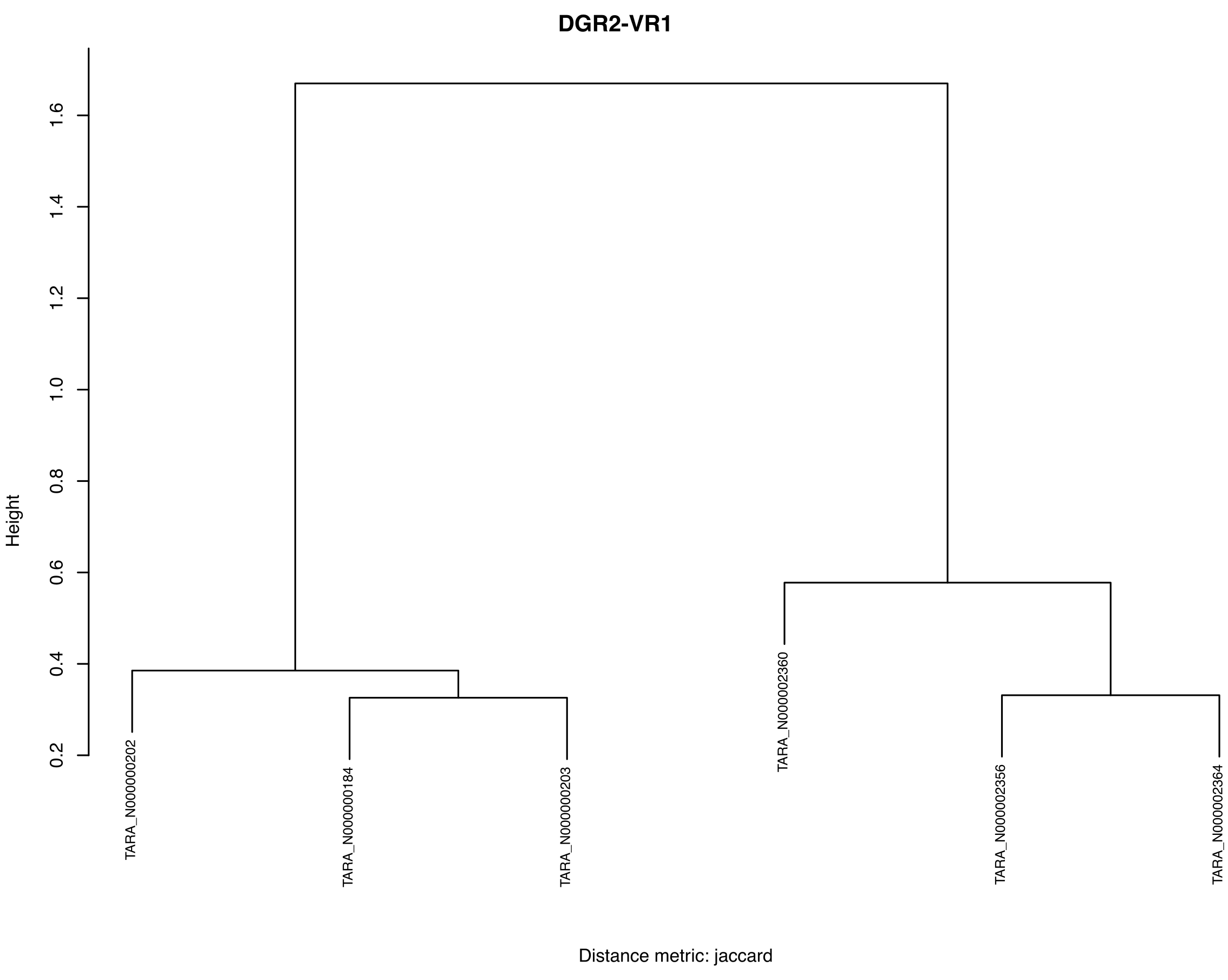
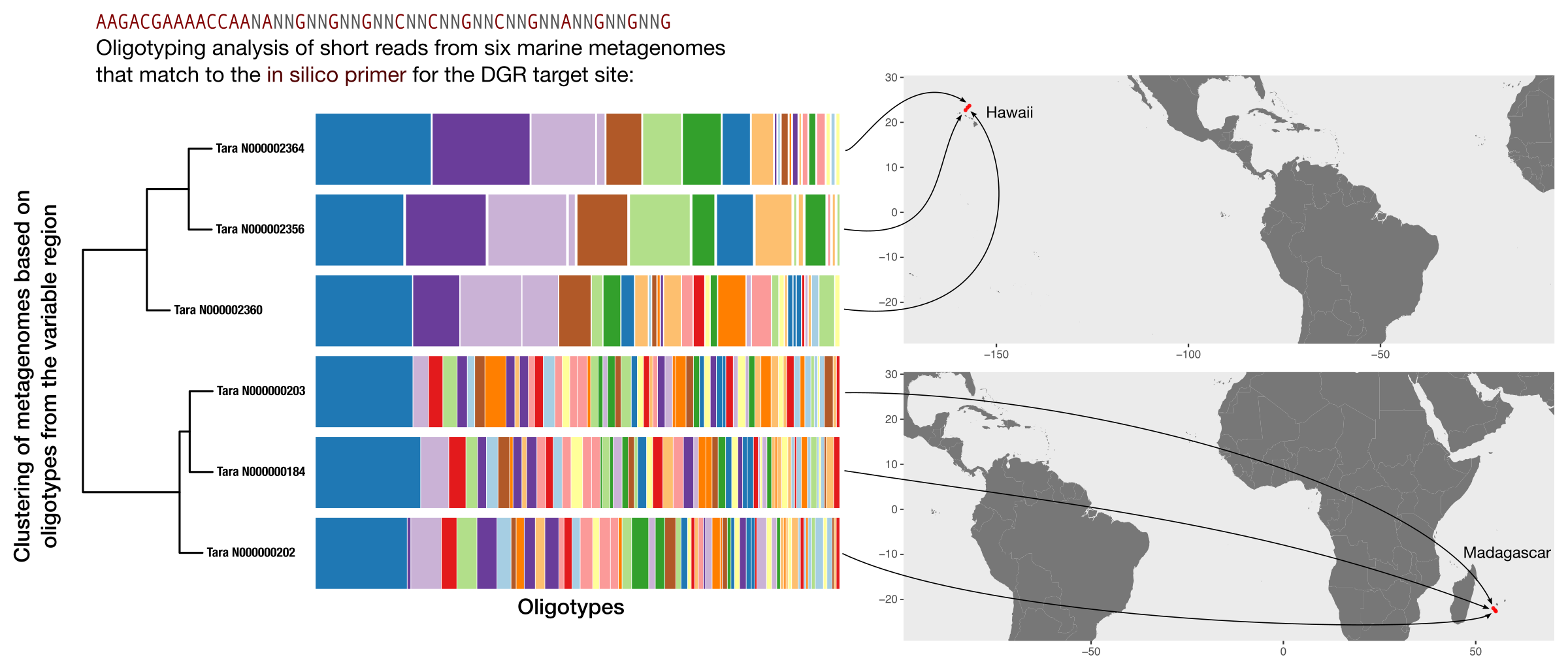
The outputs items displayed on this static web page include the following bar plot, which shows each oligotype,
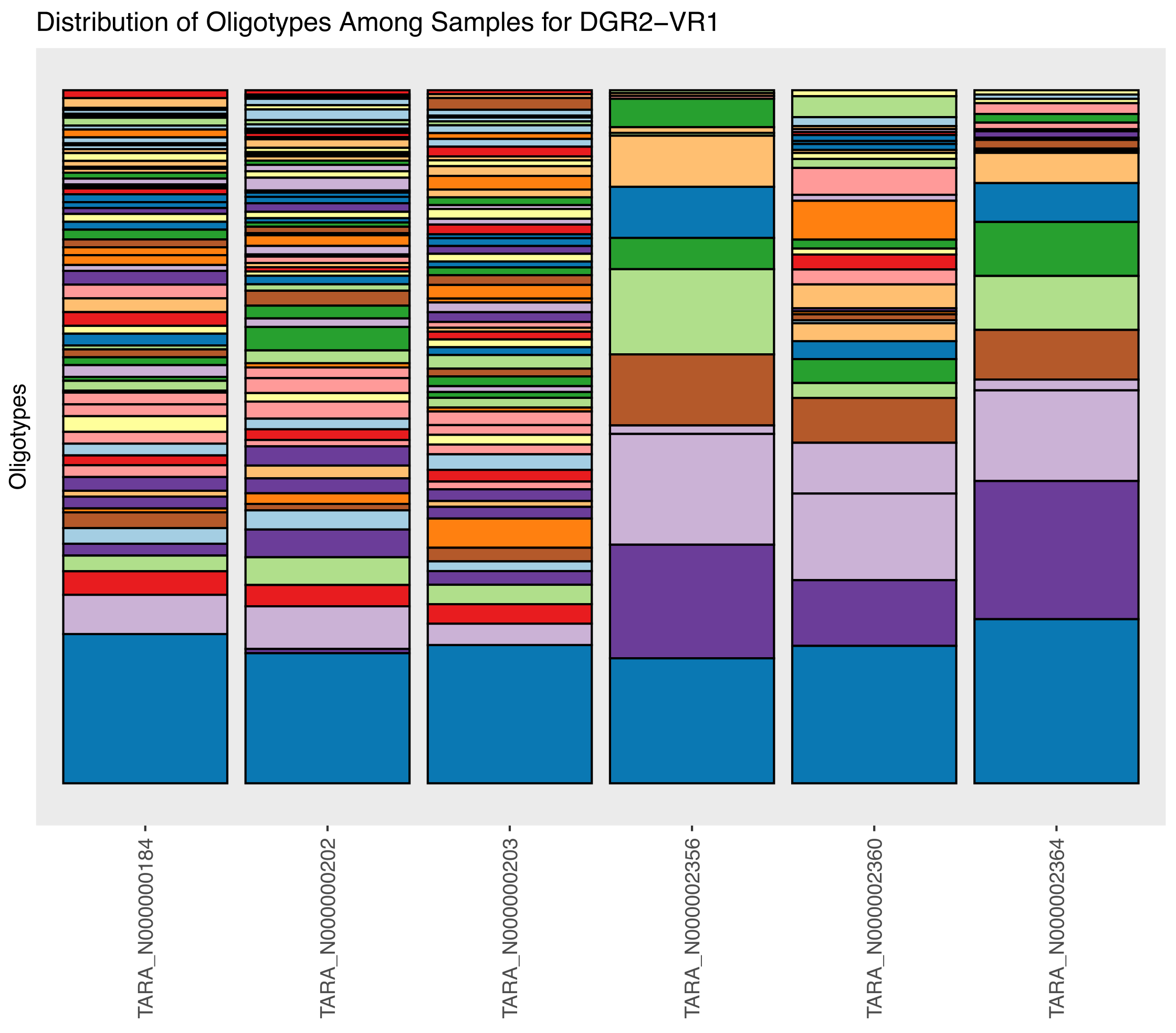
and this dendrogram, that clusters our metagenomes based on DGR-mediated sequence diversity at the variable site of the target gene one of DGR2 in the Trichodesmium erythraeum populations:
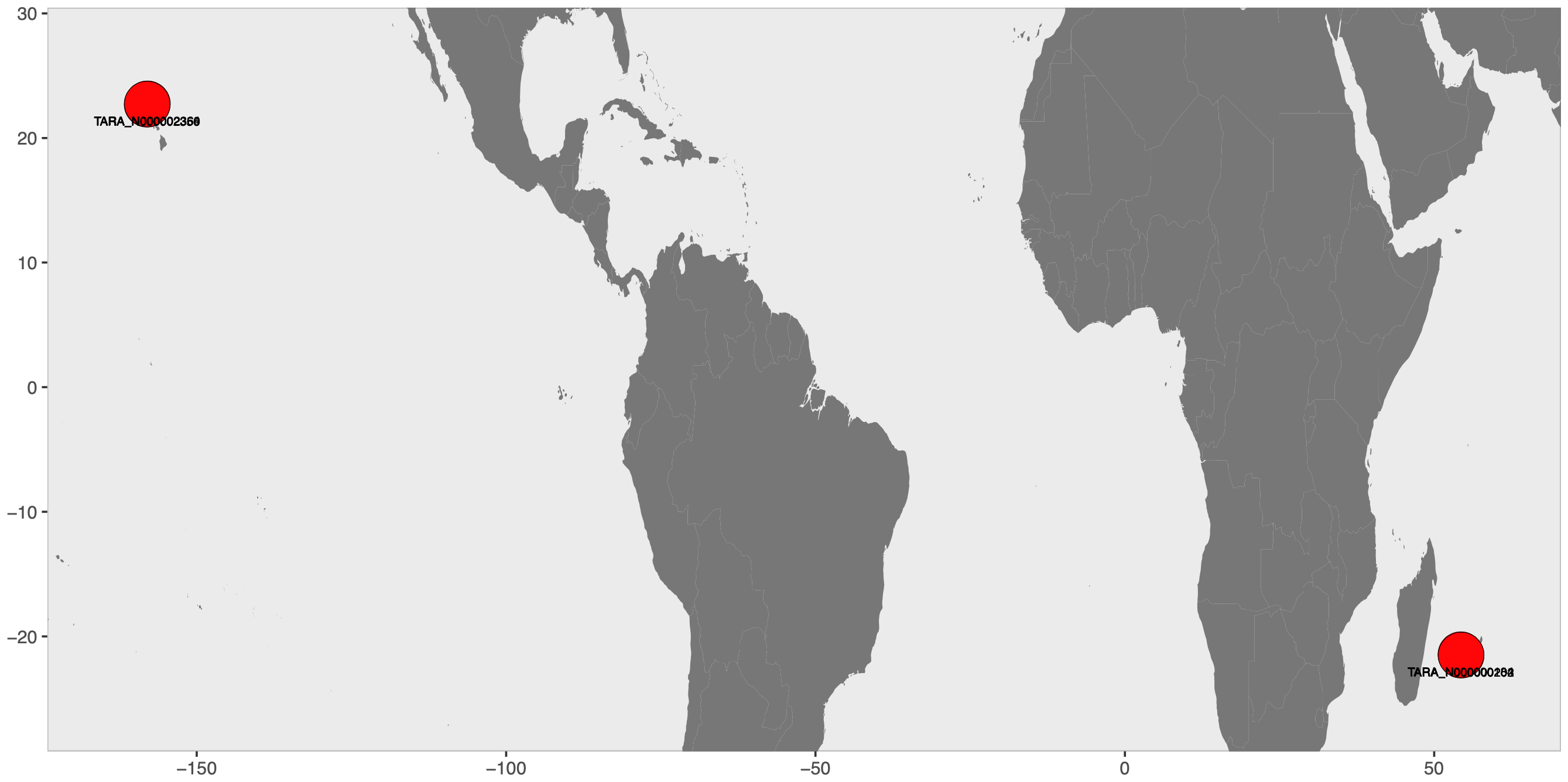
Finally, to show where these Tara Oceans Project stations are on the map, we used the library world-map-r. We first downloaded the codebase:
# get the codebase
git clone https://github.com/merenlab/world-map-r.git

# go into it:
cd world-map-r
Then replaced the contents of the data.txt with this:
| samples | Lat | Lon | MAG_MAP |
|---|---|---|---|
| TARA_N000000184 | -21.4593 | 54.3041 | 1 |
| TARA_N000000202 | -21.5043 | 54.3563 | 1 |
| TARA_N000000203 | -21.5043 | 54.3563 | 1 |
| TARA_N000002356 | 22.7091 | -158.0247 | 1 |
| TARA_N000002360 | 22.7267 | -157.9955 | 1 |
| TARA_N000002364 | 22.7511 | -157.9632 | 1 |
and run,
./generate-PDFs.R
which gave us this ugly PDF, the final piece for the Panel E of our Figure:
Then we beautified it a bit and put everything together in Inkscape:
Thank you for reading this far, and I hope this article achieved its goal to demonstrate a high-resolution approach to study within-population sequence diversity in the context of short genomic regions using metagenomics.
Please feel free to reach out to us if you are having hard time following it, or you need guidance to conduct similar analyses on your own data.
–