Table of Contents
Mapping short reads to a context is one of the essential steps of pretty much any ‘omics workflow. We are often mapping something to somewhere.
Because mapping is such a common thing we do, we made sure anvi’o can visualize mapping results so we can see what’s really going on. I know. Looking at the data. Who does that, right? Well, we have been doing it quite a lot. In fact, during the last two years we looked at reads from many different sources mapped to many different contexts. Low-coverage contigs, high-coverage contigs, good assemblies, bad assemblies, long reads, short reads, shorter reads, reads that come from low biomass samples, reads that come from high biomass samples, reads that come from out of nowhere, reads that were generated by multiple displacement amplification experiments, spit, poop, ocean, sewage, soil, and then more poop. We saw failed sequencing experiments and shared awkward moments with our collaborators, we saw non-specific mapping of short reads to unexpected contexts and had awkward moments with ourselves. We saw consistently occurring single nucleotide variants that are so infrequent in a population that made us question everything we thought we knew, and we saw single nucleotide variants sprouting all of a sudden in the context of a single gene, and we questioned everything we though we knew, again. Long story short, (1) we look at a lot of mapping results, (2) we don’t really know much. So it goes.
Despite the diversity of what one sees in mapping results, this one thing was common to pretty much all mapping results, and always made us very curious: the wavy coverage patterns.
Many times, we discussed ideas that may explain the underlying reasons for those patterns. Yet I don’t remember even a single discussion where there was a consensus that brought satisfaction and happiness. Thank you, metagenomics.
Why write about this now?
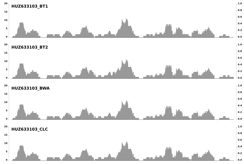
Last week I got an e-mail from Jed Fuhrman, and learned that he was also noticing these patterns and wondering about the same question. In his e-mail he mentioned that these patterns do not differ from one mapping software to another when the same set of reads mapped to the same context. Which is somewhat demonstrated in the post in which we compared 8 different mapping software. Here is just a snippet from the last image in that post to emphasize that point:
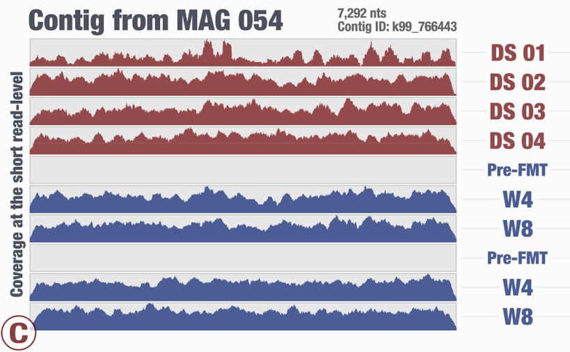
Around the same time we had just submitted the pre-print for our recent FMT study, and I again was thinking about the same thing looking at one of the figures in our study:
The next day I went to the University of Maryland to visit the Institute for Genome Sciences and Jacques Ravel’s group. During our conversations there, the same topic came up.
I thought I could write a blog post to bring this to the attention of more people, maybe to discuss if there are any ideas or opinions, and to learn from others.
I asked Jed’s permission whether I could use my response to him as a starting material, and he said OK, and here we are.
Coverage, why you do dis?
When we first implemented the ‘inspection’ function in anvi’o and started seeing these coverage patterns, I had thought that these were mostly due to some magical fluidics phenomenon happening in the sequencer or something.
But in time it became clear to us that there is much more to them than that. For instance, take another look at the second figure above. These patterns are not that random, but they are not that reproducible, either. Clearly what we observe is due to a mixture of things .. as pretty much like everything in biology.
For the sake of some formality, I will classify the factors behind variation in coverage into three major sources:
- (1) Stochastic processes
- (2) Ecologically irrelevant deterministic processes
- (3) Ecologically relevant deterministic processes
Please let me know if you don’t like any or more of these classes even after you read the following sections.
Stochastic processes
By stochastic precesses I mean really random stuff. Things that have nothing to do with anything we are doing.
At some point I wrote a very simple program that took a contig, and calculated “how many reads should I generate so the coverage of this contig would be X?”. Divide the length of the contig by the length of the desired short read length, and multiply it by the desired coverage, X. Quite straightforward. Then it generated as many reads as necessary by starting from a random position in the contig. This is how the mapping looks like when you map the resulting randomly generated short reads to cover a contig with 50X coverage:
Interesting, right?
There are already waves even when the process that generates the reads is absolutely random. This should get smoother and smoother with increasing coverage when the read length is fixed, and decreasing read lengths when the coverage is fixed.
What is simulated here may be analogous to the process that is responsible for shearing the DNA pre-sequencing. But stochastic processes can’t be all there is, because separately processed metagenomes often create similar waves when they are mapped to the same context. So there must be more.
Ecologically irrelevant deterministic processes
Some of these waves can emerge as the byproducts of the processing of the DNA before or during sequencing. I.e., the way the DNA is size-selected, or the way it is amplified on the plate during the cluster formation step pre-sequencing.
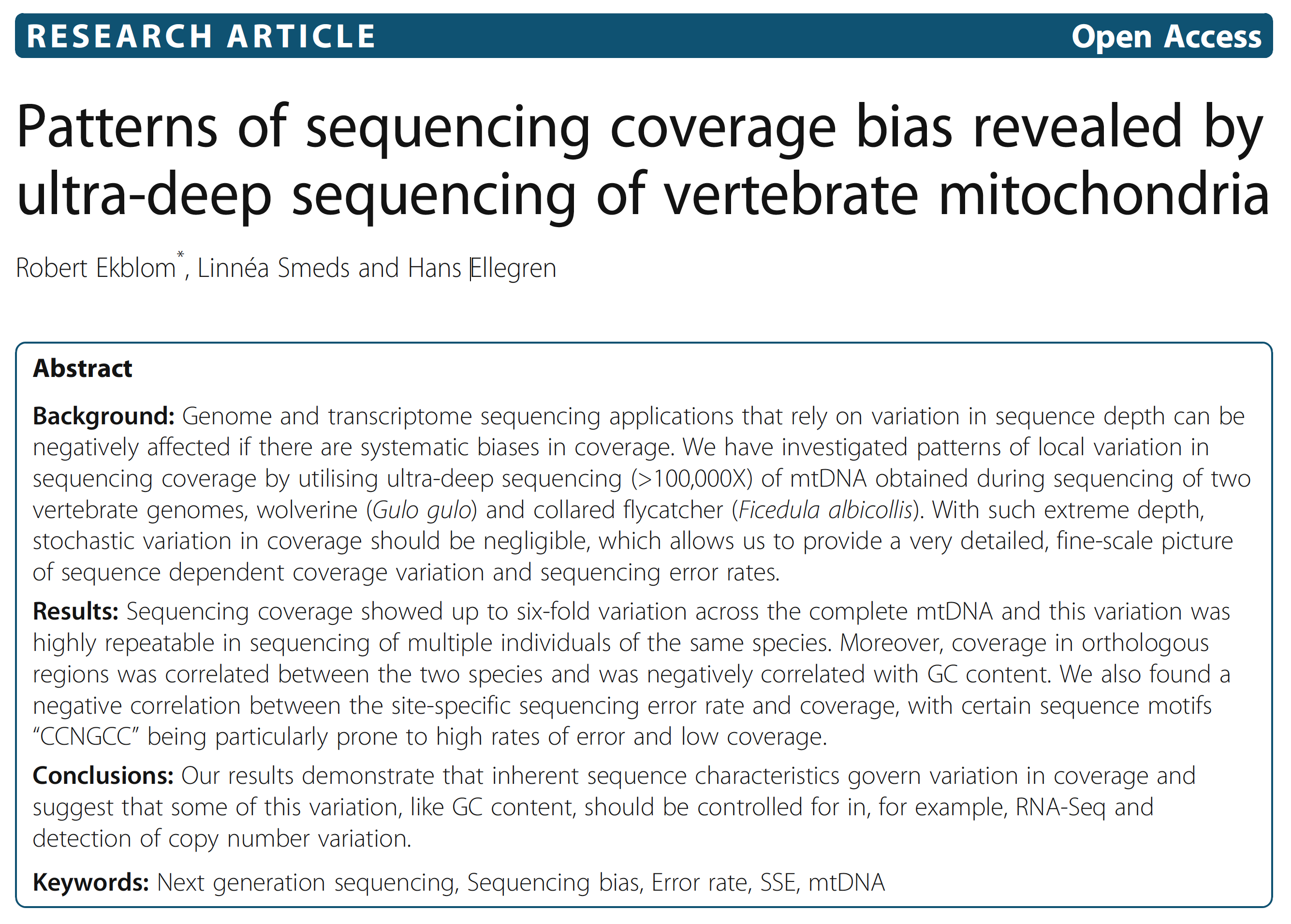
But most importantly, the basic chemical properties of DNA plays a role. For instance there is a relationship between GC-content and coverage that have been shown many times before, and people even proposed ways to correct it de novo post-sequencing (I thank Mike Love for pointing this one out). Although it is very insightful to read such studies, I haven’t yet seen a study that considers or addresses issues that arise from the complex nature of metagenomic data, and tells me that there may be more to be done in this front. Here is an interesting paper from Ekblom et al. demonstrates the GC-bias driven coverage variation in the context of Mitochondrial DNA:
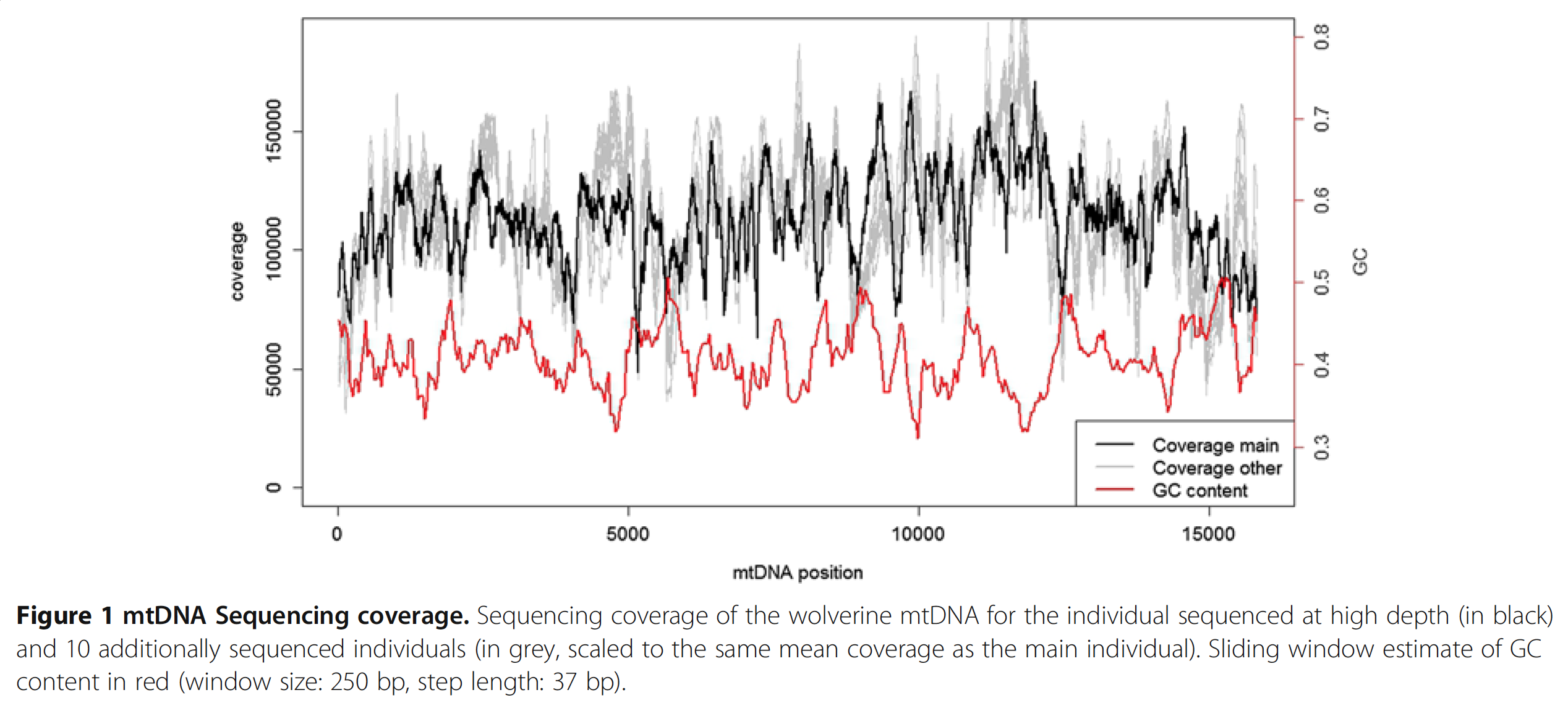
In this study authors perform a very deep sequencing of mtDNA, and find 6-fold coverage variation across the genome, which is reproducible across multiple individuals. Here is a nice figure from the paper that shows the dramatic change in coverage throughout the contig (the black line) with respect to the change in GC-content (the red line):
Well, probably no one should be surprised.
At this point I am convinced that everything in biology is either explained by GC-content, or temperature.
Of course the question is to what extent the GC-content explains the variation we see. So I did some coding today to go back to the Infant Gut dataset. Well, even though now you know what I think about biology and GC-content, I have to admit that I still was quite surprised to see that GC-content did explain quite a lot of the variation in the infant gut bins.
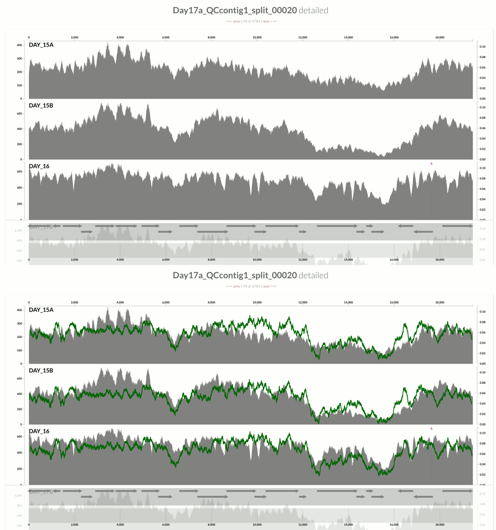
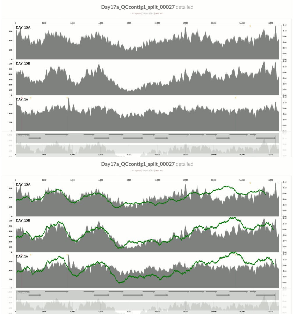
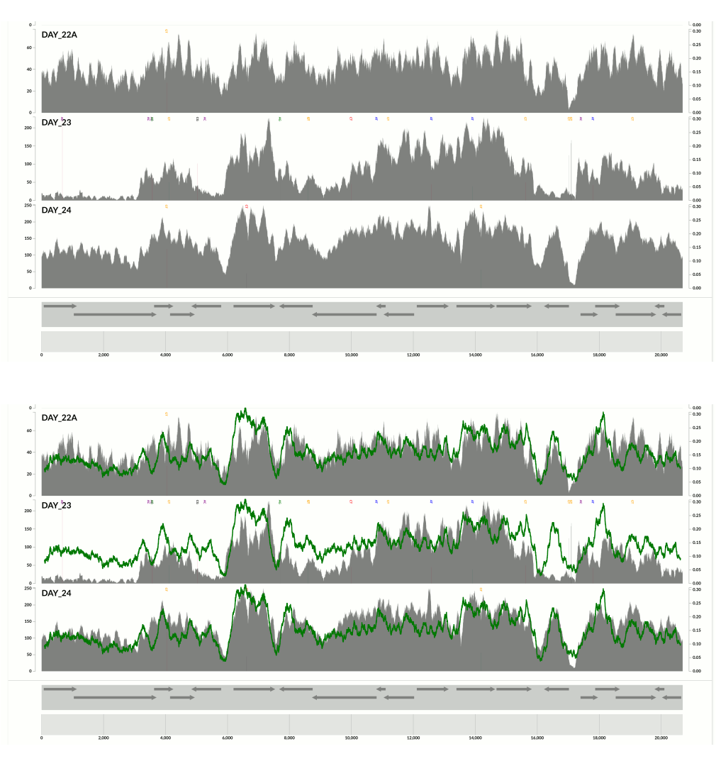
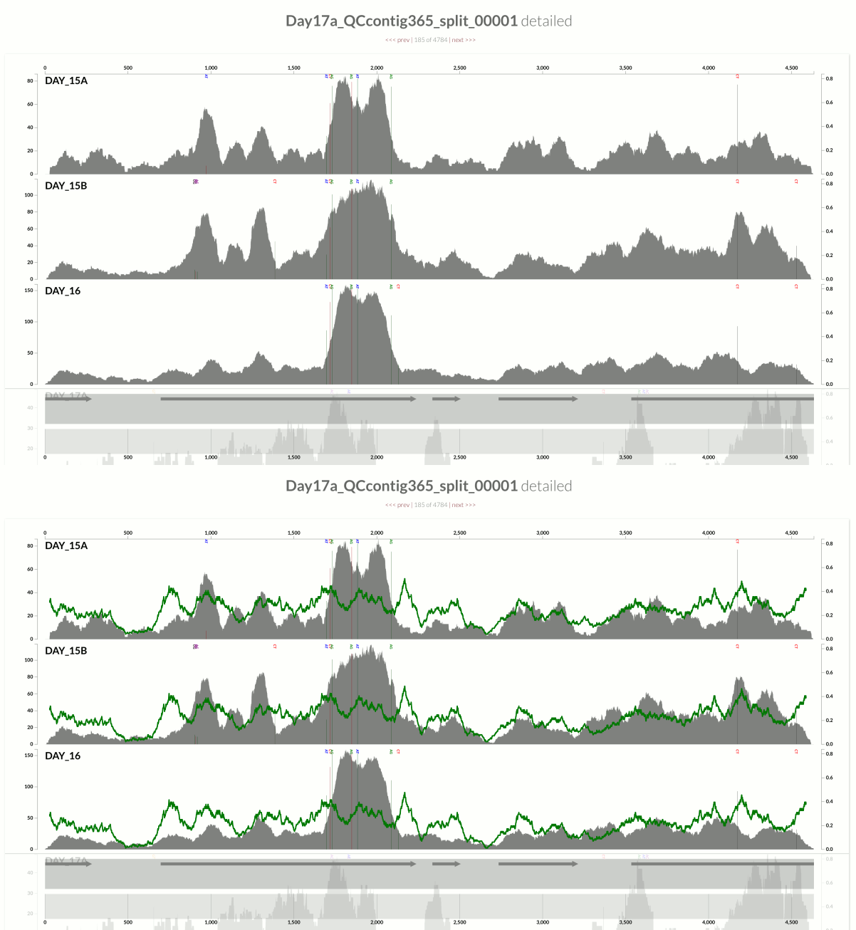
I wanted you to see it too, so I simply overlaid GC-content of the context over the coverage values. In the following example, the green line represents the GC-content (I simply shifted a sliding window one nt at a time to calculate the change in GC-content of the context):
You see it, right? Here is another one:
This one is very interesting:
Because at this point we know that Sharon et al. had used two different library preparations to generate this data. One for even days, and one for odd days. If you look closely, you can see that the GC-content explains the variation in coverage much better for even days.
The variation is equally crazy with the odd day sample, but whatever bias was introduced by the library preparation protocol used for the odd days cares a bit less about GC-content than the other one.
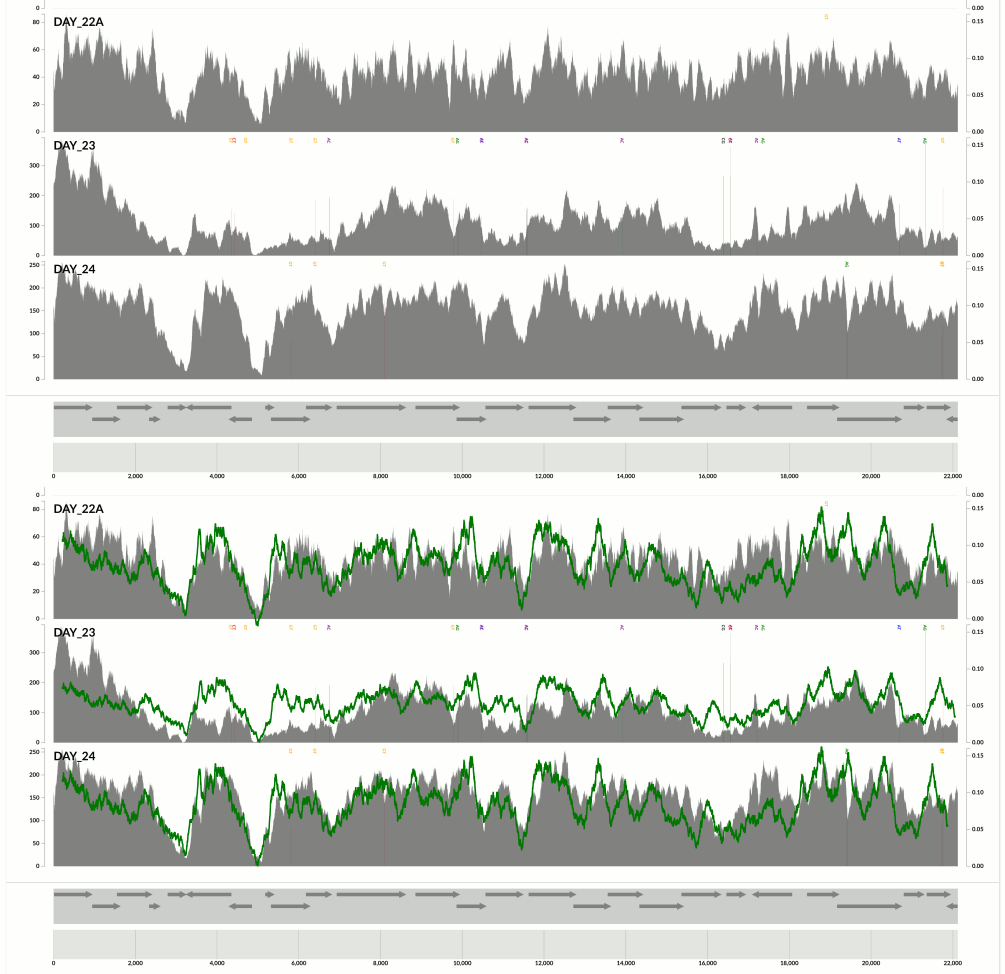
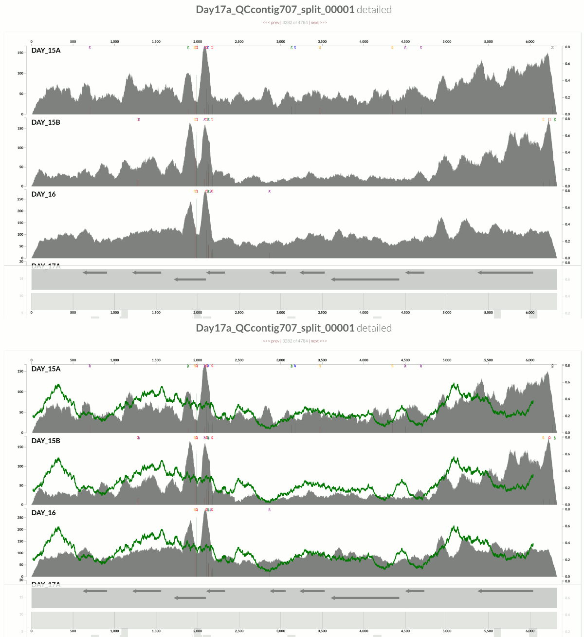
Yet another one from the same population above:
Here I confirm Ekblom et al’s findings in the context of metagenomics. They mention 6-fold coverage difference. In the last figure I see 10-fold coverage difference.
One thing that needs to be clarified is how specific is the emergence of these patterns to the library preparation protocol. I just realized that we should visualize these lines for every contig in the inspection page of anvi’o. Maybe if it is so available, we can collect more reports and start seeing how these patterns play out with different environments, protocols, etc.
But just think about the implications of these variations in binning based on abundance / coverage.
Besides GC-content, biases that result in variation in coverage also stem from running MDA, or too many cycles of PCR on low input biomass, which usually produce coverage profiles that look like city skylines. I guess these can be put in this category as well. But the take home message from this limited data is most of those waves come from GC-rich and GC-poor areas of the genome.
Ecologically relevant deterministic processes
It seems that, at least based on the data we have in this post and the Ekblom et al. publication, the GC-content drives a lot of things, but ecology will once in a while sing the song of its people, too.
The ecologically relevant processes to the variation in coverage is mostly manifested by ‘non-specific mapping’. There are different types of non-specific mapping that I will not try to describe here. Instead I will give two examples, and maybe come back later to refine them (because I have a workshop to give tomorrow, and I really need to sleep).
Most metagenomic assemblies will recover only a subset of genomes that occur in the actual sample. During the mapping,the short reads from viral, bacterial, archaeal, or eukaryotic genomes that are not represented in the assembly will end up being mapped to some of the available target contigs whenever there is enough sequence conservancy.
Non-specific mapping occurs when short reads map to a context from which they do not originate. You can imagine that the coverage around regions that are conserved across multiple populations would have a higher coverage in general. This is a more complex problem than it sounds, but regardless of the extent to which we can explain it in detail, the rate of non-specific mapping in a project does tie back to the ecology.
We have seen during the last two years that in some cases the variation of coverage looks like ripples on a lake, in other cases it resembles choppy waters in the ocean, and sometimes the structures in the Grand Canyon.
I think it would make intuitive sense to a lot of people that the larger the amount of sequences in a metagenomic library is explained by the assembly (or the ‘context’), the more ‘calm’ this pattern would become. While the variation in coverage for good assemblies (or more complete representative context) will mostly be impacted by (1) (stochastic processes) and (2) (the ‘ecologically irrelevant deterministic processes –like GC-content), for worse assemblies it will be impacted by the first two, as well as (3) (the processes that are relevant to ecology).
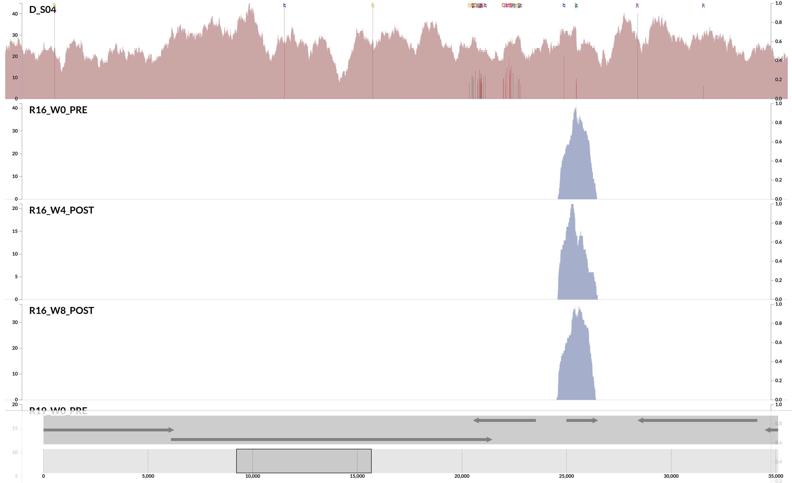
Here is a very clear, and a very extreme example of ‘non-specific mapping’:
This is from our FMT study. As you can see, the population that is present in our donor sample D_S04 is not detected in the recipient pre- or post-FMT. Yet, somewhere in the recipient metagenome that one tiny gene is present, and short reads are being recruited to its context from those samples. This happens quite often and in more subtle ways, and contributes to the variation in different ways. I guess we can agree that the variation of coverage we observe in the recipient samples is completely due to (3) in this extreme case.
Let’s take a look at another type of complexity that results in a different type of non-specific mapping.
Indeed, the context I keep mentioning does not have to be the contigs from a metagenomic assembly. You may map reads to an isolate genome, too. In a sense, mapping reads from an isolate back to the isolate is the positive extreme of how representative a context can be since the vast majority of reads, if not nearly all of them, will end up mapping to the context they come from. In this situation ecologically relevant factors for variation in coverage will have no impact, and most of the variation will emerge from (1) and (2). Here is a reminder of how a contig from a nearly monoclonal E. facealis population in a very simple metagenome looked like:
The impact of anything ecologically relevant is virtually absent while the variation is largely explained by the GC-content.
In contrast, here is an example from another population from the same metagenome:
This one demonstrates something that is closer to the opposite extreme, where the variation in coverage is mostly due to (3). This contig happens to belong to the S. epidermidis ‘pangenome’, so it is much more likely to have mapping of reads emerging from more than one population of S. epidermidis (Sharon et al. had eloquently described the occurrence of multiple ‘strains’ of S. epidermidis, and we had shown in the anvi’o methods paper the recovery of single-nucleotide variation patterns from these populations (here is a direct link to the relevant figure)).
Take a look at the high-coverage part of the contig, which coincides with the second half of that gene. This high-coverage area also contains multiple single-nucleotide variants, which indicates short reads that originate from slightly differing contexts are being mapped to this part of the contig. Although GC-content is not completely irrelevant for some parts of the contig, it completely fails to explain some of the patterns of variation. Here is another example from the same population:
Let me state the obvious just to have it in writing:
We learn two things from these. One, the variation of coverage in the S. epidermidis contigs demonstrate to what extent the factors related to the ecology can impact the mapping outcomes. So non-specific mapping can be a real burden for accurate insights into population dynamics. Two, the intriguing difference in variation of coverage between the S. epidermidis and E. facealis contigs suggests that the dynamics affecting different populations can differ dramatically even in the same dataset.
These shouldn’t surprise any microbiologist. But, seeing them this way makes one wonder about all the potential pitfalls in our workflows that may deny us from accessing to various populations for reasons that are relevant to their ecology.
Final words and summary
There are stochastic and deterministic factors that affect the coverage.
Deterministic factors include things that are irrelevant to ecology of populations, such as GC-content, and things that are relevant to ecology, such as non-specific mapping.
Non-specific mapping is the worst. We hate it. The amount of non-specific mapping differs from environment to environment, or due to changes in the complexity of a community over time. Maybe we can model the non-specific mapping patterns in an attempt to better understand something about the ecology of the environments we are studying. I think there is a lot to be done here.
GC-content. We love GC-content. But it is also very sad that there is such a strong bias with it. This bias not only diminishes the efficacy of contig abundances for binning, but also limits our ability to recover single-nucleotide variants from GC-poor regions of population genomes we study. If the GC-content bias is so reproducible, we can normalize coverage values to improve binning or other practices that rely on coverage values. However, I remind myself that if we want to take that route we need to have a broader look at how different library preparation, and amplification methods affect the magnitude of bias.
Besides its toll on binning, you can see that relying on gene average coverage values to study the functional potential of a given community may require some extra attention since it seems the coverage can change as much as an order of magnitude between GC-rich and GC-poor regions of the same contig of the same population genome.
Anvi’o can and should do a better job visualizing these patterns across contigs, so we can slowly develop a knowhow as a part of our daily exploration.
Now you have all my 2 cents.
Over and out.
Have you also been curious about wavy coverage patterns in mapping results? Good! Here is a blog post on that: https://t.co/ZspVAjhtUS
— A. Murat Eren (@merenbey) December 15, 2016


