


Table of Contents
Mapping short reads to contigs is one of the most critical steps of the assembly-based metagenomic workflow. Because the number of mapped reads define the mean coverage for each contig, mapping provides the crucial input for clustering algorithms that use coverage patterns of contigs across samples to identify genome bins. The appropriate mapping is important, therefore the mapping software, and the stringency.
During our discussions to identify which mapping software should we use to map short metagenomic reads to contigs, Bing Ma (the Department Microbiology and Immunology, University of Maryland), suggested that it would be wise to compare multiple of them to make an informed decision instead of just picking our favorite.
However, comparing the efficiency of mapping software is not an easy task if you want to do it with “real world” data. We used eight mapping software to map short reads back to a metagenomic assembly, and profiled mapping results using anvi’o. Here you will find a brief overview of our findings. However, I would like to remind you early on that this by no means is an exhaustive comparison of these software, and our results are only meaningful within the narrow parameter space we explored. To avoid a biased comparison, we chose parameters from author-suggested defaults.
But beyond our preliminary findings on the performance of these mapping software, this little project gives a good idea about how versatile anvi’o is as a platform, and its potential use as a benchmaraking environment.
Preparation
First a bit information about the dataset. We used one of Jacques Ravel’s not-yet-published datasets with his permission. Let’s call it HUZ63.
HUZ63 is a dataset of four vaginal metagenomics generated from sampling of the same individual in four time points. Bing pulled all short reads together from all four samples, co-assembled them using IDBA-UD to acquire the “community contigs”, and then mapped short reads back from individual samples to these contigs using 8 mapping software:
Details of each algorithm is beyond the scope of our little study, however, the user’s control over the mapping stringency changes from one another. You can find more information about each of them in the links above.
Bing Ma kindly shared her BASH script that describes how all these mappers were run (this part is for code-savy people who may like to do a similar analysis themselves, others should feel free to skip):
#!/bin/bash

#not all variables defined below would be used in all aligner
sample= # sample name
ref=  # give it a reference database name
query= # query fasta file
reffas= # reference fasta file name
datadir= # where the original fastq file stored
output_dir= #final output directory

#bbmap, when give the reference, it generate the reference db on the fly
bbmap.sh ambig=all ref=$reffas in=$query outm=$sample.bbmap.bam

##bowtie v1, I put down the input files as paired-end sequences and the unpaired single reads
zcat $datadir/{${sample}_pe_1.fastq.gz,${sample}_pe_2.fastq.gz,${sample}_se.fastq.gz} | bowtie -p 16 -l 22 --fullref --chunkmbs 512 --best --strata -m 20 -n 2 --mm $ref -S - | samtools view -bS - > $sample.bt1.bam

#bowtie2, first build reference db, then perform mapping
bowtie2-build $reffas $sample
bowtie2 -x $ref -f $query -S $sample.bt2.sam
samtools view -bS $sample.bt2.sam > $sample.bt2.bam
rm $sample.bt2.sam

#BWA, create db first
bwa index -p $ref -a bwtsw $reffas
bwa aln $ref $query > $sample.sai
bwa samse -f $sample.bwa.sam $ref $sample.sai $query
samtools view -bS $sample.bwa.sam > $sample.bwa.bam
rm $sample.sai $sample.bwa.sam

#gsnap
gmap_build -d $ref -D $output_dir $reffas
gsnap -A sam -d $ref $query -D $output_dir | samtools view -bS - > $sample.gsnap.bam

#novoalign
novoindex $ref $query
novoalign -r Random -o SAM -f $query -d $ref | samtools view -bS - > $sample.novoalign.bam

#smalt
smalt index -k 13 -s 6 $refname $reffas
smalt map -f sam -o $sample.smalt.sam $ref $query
samtools view -bS $sample.smalt.sam > $sample.smalt.bam
rm  $sample.smalt.sam
The result of this script was 8 BAM files for each sample, where identical short reads were mapped to identical contigs.
When Bing sent me the total of 32 BAM files for HUZ63 along with the contigs, I used anvi’o to (1) generate an contigs database and annotate contigs using myRAST, (2) run HMM profiles for single-copy gene collections on this database, (3) profile each BAM file with -M 2000, (4) merge the ones that are coming from the same mapper first, (5) and finally merge everything together using (the user tutorial details these standard steps of the metagenomic workflow we implemented in anvio).
Here is the the shell script I used for all these steps, again, for people who may want to do a similar analysis in the future (or for the ones who want to familiarize themselves how does anvi’o look like in the command line (of course it is simplified, since each step was sent to clusters in the original one)):
#!/bin/bash

# this is how the directory in which I run this script looked like:
#   $ ls *bam
#   HUZ633103.bbmap.bam      HUZ634093.bbmap.bam      HUZ635444.bbmap.bam      HUZ636473.bbmap.bam
#   HUZ633103.bt1.bam        HUZ634093.bt1.bam        HUZ635444.bt1.bam        HUZ636473.bt1.bam
#   HUZ633103.bt2.bam        HUZ634093.bt2.bam        HUZ635444.bt2.bam        HUZ636473.bt2.bam
#   HUZ633103.bwa.bam        HUZ634093.bwa.bam        HUZ635444.bwa.bam        HUZ636473.bwa.bam
#   HUZ633103.clc.bam        HUZ634093.clc.bam        HUZ635444.clc.bam        HUZ636473.clc.bam
#   HUZ633103.gsnap.bam      HUZ634093.gsnap.bam      HUZ635444.gsnap.bam      HUZ636473.gsnap.bam
#   HUZ633103.novoalign.bam  HUZ634093.novoalign.bam  HUZ635444.novoalign.bam  HUZ636473.novoalign.bam
#   HUZ633103.smalt.bam      HUZ634093.smalt.bam      HUZ635444.smalt.bam      HUZ636473.smalt.bam
#   contigs.fa
#
# Remember that this is a simplified version of the original script. Each section in this script can be
# (and should be) 'clusterized' to run it parallel. Otherwise, considering the fact that those nested
# for loops run 32 times, it would take forever even for a small dataset.

set -e

samples="HUZ633103 HUZ634093 HUZ635444 HUZ636473"
mappers="bbmap bt1 bt2 bwa clc gsnap novoalign smalt"

######################################################################################################################
# GET RAST ANNOTATION
######################################################################################################################

svr_assign_to_dna_using_figfams < contigs.fa > svr_assign_to_dna_using_figfams.txt


######################################################################################################################
# INIT BAM
######################################################################################################################

for mapper in $mappers
do
    for sample in $samples
    do
        mv $sample.$mapper.bam $sample.$mapper-raw.bam
        anvi-init-bam $sample.$mapper-raw.bam -o $sample.$mapper
    done
done


######################################################################################################################
# CONTIGS
######################################################################################################################

# GEN CONTIGS FOR ALL
anvi-gen-contigs-database -f contigs.fa -o contigs.db

# ANNOTATE WITH RAST
anvi-populate-genes-table contigs.db -p myrast_cmdline_dont_use -i svr_assign_to_dna_using_figfams.txt

# POPULATE SEARCH TABLES
anvi-run-hmms contigs.db


######################################################################################################################
# PROFILE
######################################################################################################################

for mapper in $mappers
do
    for sample in $samples
    do
        anvi-profile -i $sample.$mapper.bam -o $sample.$mapper -c contigs.db -M 2000
    done
done


######################################################################################################################
# MERGE INDIVIDUAL SAMPLES
######################################################################################################################

for mapper in $mappers
do
    anvi-merge *.$mapper/RUNINFO.cp -o $mapper-MERGED -c contigs.db
done


######################################################################################################################
# MERGE EVERYTHING
######################################################################################################################

anvi-merge */RUNINFO.cp -o ALL-MERGED -c contigs.db
When this script was done running, I had 9 merged anvi’o profiles (one for each mapper + one for all):
$ ls -d *MERGED
ALL-MERGED    bt2-MERGED  gsnap-MERGED
bbmap-MERGED  bwa-MERGED  novoalign-MERGED
bt1-MERGED    clc-MERGED  smalt-MERGED
A quick first look and initial binning
Having read this FAQ, I knew Bowtie (bt1) was going to offer a pretty decent mapping. So I visualized Bowtie results initially to describe this dataset and samples in it.
I run anvi-interactive from the terminal to start the interactive interface:
anvi-interactive -c contigs.db -p bt1-MERGED/PROFILE.db
And did some quick supervised binning (which took about four mouse clicks). Here is a screenshot from the interactive interface that shows my selections:
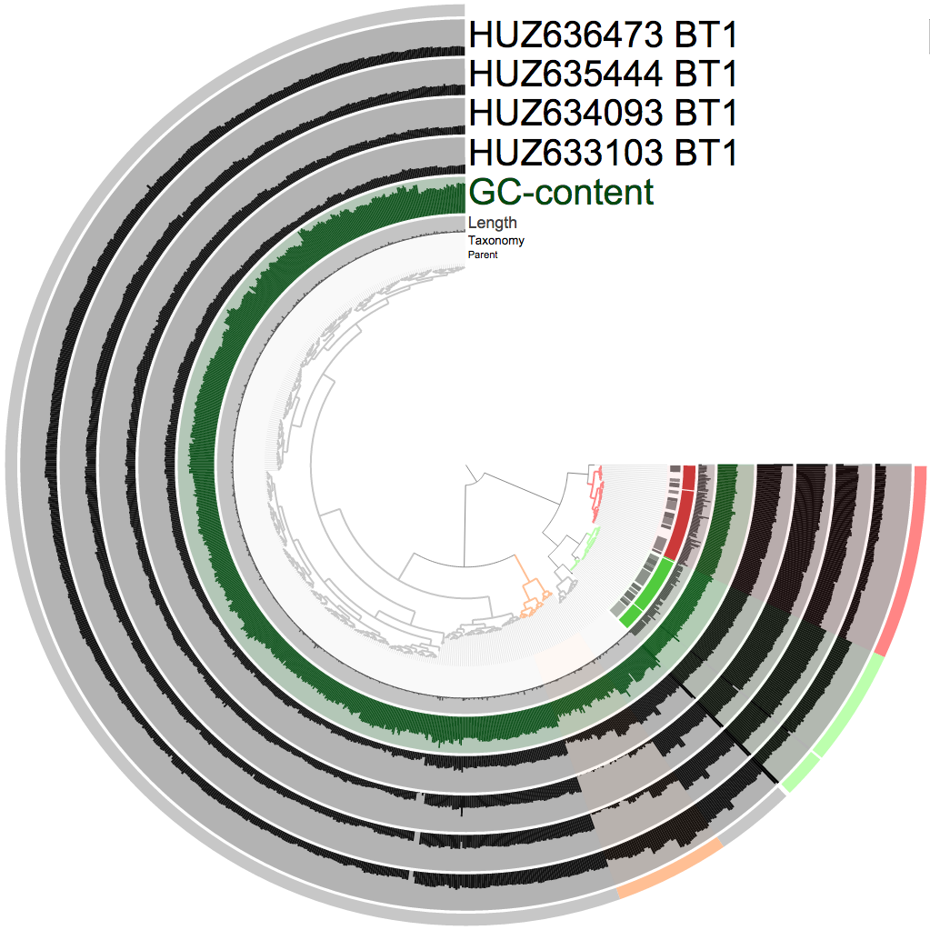
In case you are not familiar with this view here is a crash course: the tree in the center shows the organization of contigs based on their sequence composition and their coverage across samples (which is one of anvi'o's multiple default clustering algorithms). Every bar in each black layer shows the coverage of a given contig, in a given sample. There are some extra layers betwen the tree and samples in this particular screenshot: parent (if a contig was too long and soft-broken into multiple splits this layer will show gray bars connecting the ones that are coming from the same mother contig), taxonomy (the consensus taxonomy for proteins identified in a given split, contributed by myRAST annotation), and GC-content (computed directly from the contigs themselves during the creation of the contigs database). The most outer layer describes my selections (when I click on a branch, it adds them to a bin, later I change the color; and clicking a branch is something like [this](http://g.recordit.co/kyupW8Yyu7.gif)).
The RAST taxonomy (the second most inner circle) already identifies every single bacterial contig in this very simple community. They are also clustered very nicely into separate clusters, so binning them is quite straighforward. The remaning contigs are coming from two sources. The first source is Trichomonas vaginalis (represented by the orange selection), a protozoan that causes trichomoniasis. Although it was a pretty obvious cluster (note the change in coverage across time points), there was no evidence from myRAST regarding taxonomy. Yet, when I BLAST-searched multiple contigs from that group randomly, all of them hit T. vaginalis genomes on NCBI with very high accuracy. The distribution patterns of these contigs are identical, so they are very likely to be coming from one genome. Although within the cluster there are multiple “levels” of stable coverage, which I didn’t try to find an explanation for. There may be multiple T. vaginalis organisms at different abundances, or there may have been other reasons that I can’t think of right at the moment that are affected different parts of this eukaryotic genome differently and made them more or less present in the sequencing results due to some biases occured during the extraction or sequencing.. The second source for the remaning non-bacterial contigs was the host genome (the gray selection). Which is quite clear as the coverage does not change across time points for these contigs (it is nice to see that in a weird way, because it gives me a bit more confidence in DNA extraction and sequencing technologies that in general I am extremely sceptical about (so how about the irregularity with *T. vaginalis?* (well, OK, except that))).
After storing these bins as a “collection” from the interface, I clicked the “generate summary” button, and got a static HTML output with all sorts of information about them. I am not going to share the entire output, but here is a screen shot from one of the panels to give a brief idea about what we have:
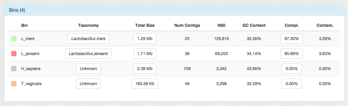
In less than a minute, two near-complete bacterial genomes (and tiny chunks from a ~160 Mbp protozoan genome). Not bad.
OK. Now we have an overall understanding of the dataset, and we performed a reasonable binning using the Bowtie output (so we know which contig belongs to what group).
Number of mapped reads by each mapper
There is more to do, but first I would like to get a quick understanding of how many reads mapped to these contigs by each mapping software. Since we are mapping same reads to the same contigs across the board, the numbers should be quite similar to each other in an ideal world.
Fortunately the number of mapped reads is stored in the self table in every profile database anvi’o generated. An anvi’o profile database can simply be queried like this from the command line:
$ sqlite3 HUZ633103.bbmap/PROFILE.db 'select value from self where key = "total_reads_mapped";'
5655338
So I write a tiny loop to generate a csv file with the number of maped reads from each mapper:
counter=0;
for m in bbmap bt1 bt2 bwa clc gsnap novoalign smalt
do
    num_reads=`sqlite3 HUZ633103.$m/PROFILE.db 'select value from self where key = "total_reads_mapped";'`;
    counter=$((counter+1));
    echo $counter $m $num_reads
done > x.csv
And a hacky one-liner for a quick visualization of this file (which now contains the number of mapped reads from each mapper):
$ echo "set boxwidth 0.5;\
>       set logscale y;
>       set style fill solid;
>       plot '-' using 1:3:xtic(2) with boxes" \
>          | cat - x.csv gnuplot -p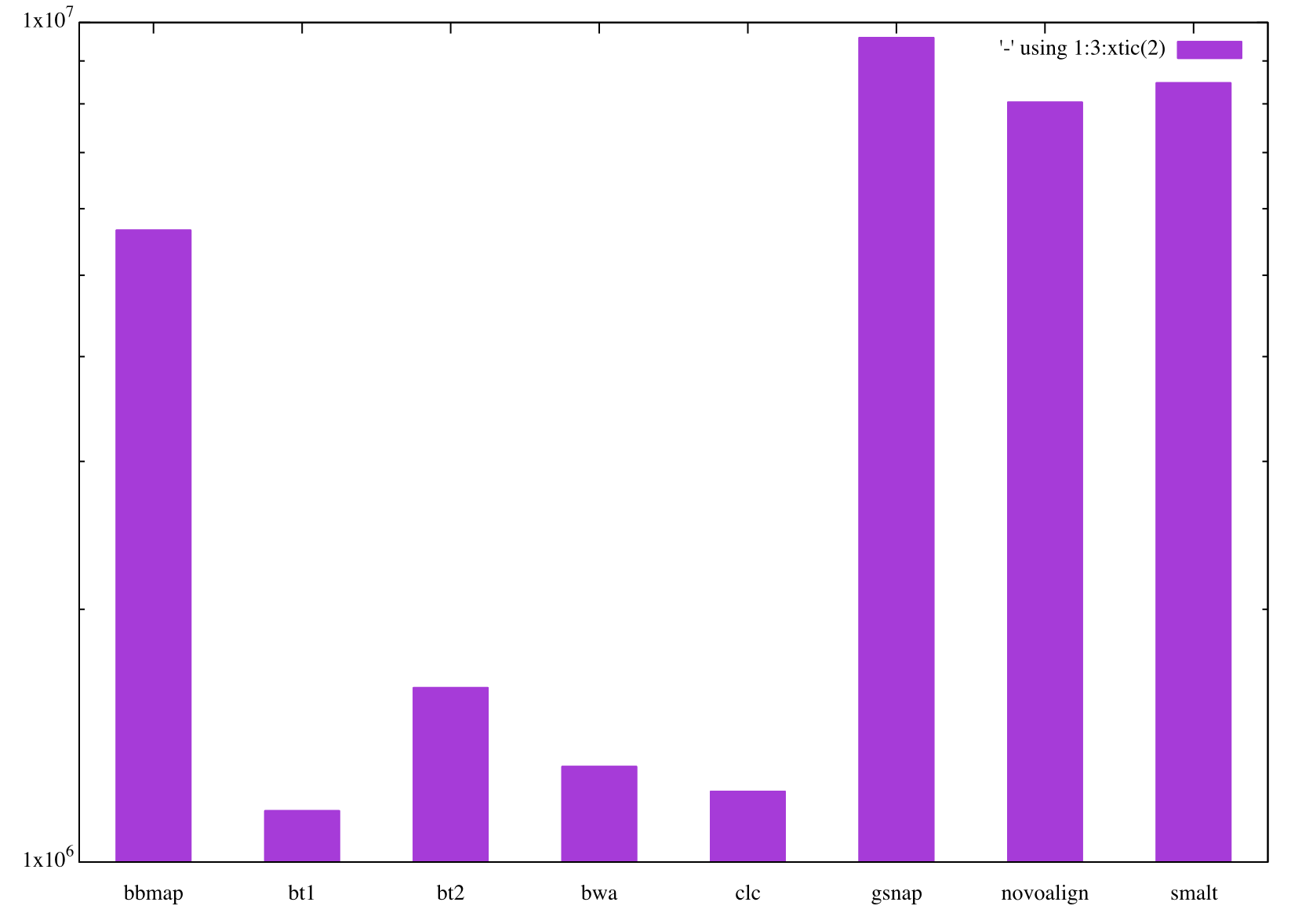
So the number of reads mapped by each mapper is not really “identical”. Note the log-scale for the Y-axis. So in fact they are far from being similar. Interstingly, two groups of mappers emerge from this. One group, that maps crap loads of reads to these contigs, which include BBMAP, GSNAP, SMALT, and Novoalign, and the second group that maps much smaller number of reads in comparison to the first one which include Bowtie, Bowtie2, BWA and CLC. We say “OK”, and continue.
Comparing individual mapping results
In an ideal situation, the organization of contigs in this dataset based on coverage values, and therefore the selections I made using Bowtie should be identical across different mappers.
For instance, wouldn’t that be great if I could fire up the interactive interface for, say, CLC results, and highlight my bins I identified in Bowtie results?
With anvi’o this is an incredibly simple task. All you need to do is to export your collection, and import it back into each profile database using anvi-import-collection.
So I visualzed each mapping result through the interactive interface, and loaded my bins I had identified using Bowtie. Here is a composit screenshot that shows you the results:
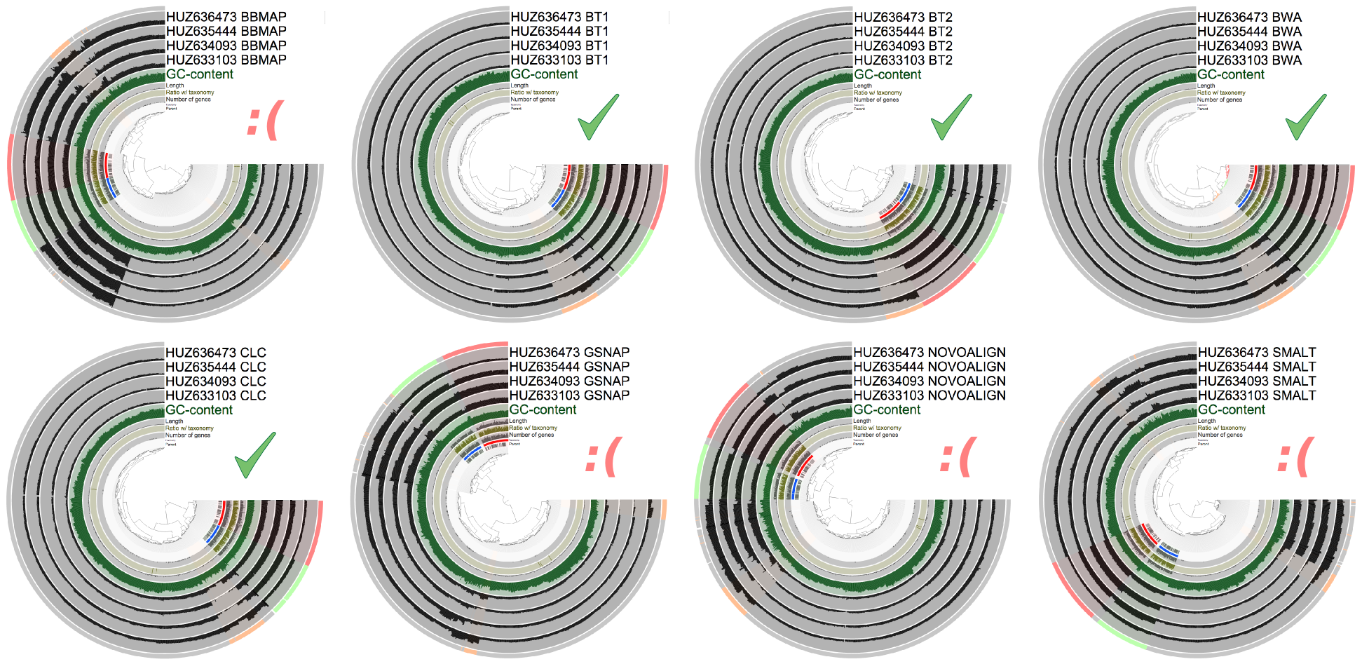
The question here is this: if I didn’t know these bins, could I have identified them in different mapping results. For some of them, the answer is a straight yes. For some others, the answer is just a partial yes.
As you can see, they all did well with bacterial genomes. Both bacterial genomes that are well assembled and covered reasonably are together, and they form two distinct clusters in trees generated for each mapping result. On the other hand, the performance of mappers change when you look at the third organism we identified, which is neither well-assembled, nor well covered: T. vaginalis. There is an OK sign for every mapping software that provided the clustering algorithm with accurate information so it managed to keep T. vaginalis contigs somewhat together. Others, didn’t do as well, and T. vaginalis contigs were scattered around the tree and was mixed with host contamination.
You may wonder “why do I care? When I do mapping, I do it to find out about the bacterial genomes anyway”. Fair enough. But you must consider that T. vaginalis in this case can be seen as a poorly-assembled bacterial genome with poor coverage in a more complex dataset (which is like every other metagenomic dataset that doesn’t come from the vaginal environment), so it is important to keep T. vaginalis together.
Putting all mapping results together
OK. The previous screen does not help us much about what happens to individual splits/contigs across the tree. One contig in tree A is at 12 o’clock, and the same contig ends up somewhere around 9 o’clock in tree B. Wouldn’t it have been lovely to put all the contigs and their coverages across samples with respect to all mapping software on one tree?
Well, this also is an easy task for anvi’o. The very last line of my BASH script merges every single profile together. And this is a screenshot that visualizes the mean coverage values across the samples:
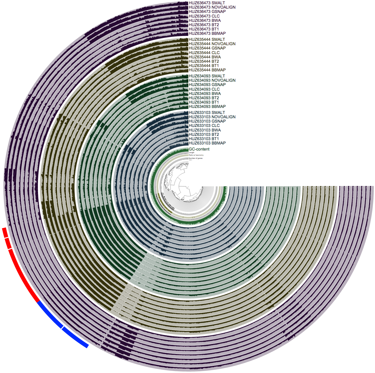
So this is a busy figure, but what it shows is pretty simple. Each sample is colored differently, and identified as a block of 8 layers. In each sample block, you see 8 mappers, and the mean coverage value estimated for a given split in that sample based on how many reads they mapped to that split. So when you pick a hypothetical leaf of the tree in the center, and follow its line towards the most outer circle, all bars you cross should have an equal size within each sample block. Because we know that the relative abundance of a given contig does not change from one layer to the other within a sample block in reality, if it seems it is changing, the only reason for it is because different mapping software do not operate on it similarly. For the bacterial part things are working pretty well, but once you get out the oasis of beautifully assembled genomes, you see a lot of disagreement between mappers.
Although now we know that the first group of mappers that map more reads to these contigs are the ones that have done poorly (simply because clustering based on their numbers split a cluster that should be one piece into multiple pieces), but we still don’t know what is it that they do wrong.
One of the natural outcomes of mapping reads on a contig as a mistake is the dramatic increase in variability at nucleotide positions. Because if you map a lot of reads to a position when they shouldn’t map there, what you get back is a lot of SNPs. Anvi’o is very helpful at exploring these variability patterns. For instance, this screenshot is the same with the previous one, but it shows the “variability” view instead of the “mean coverage” view:
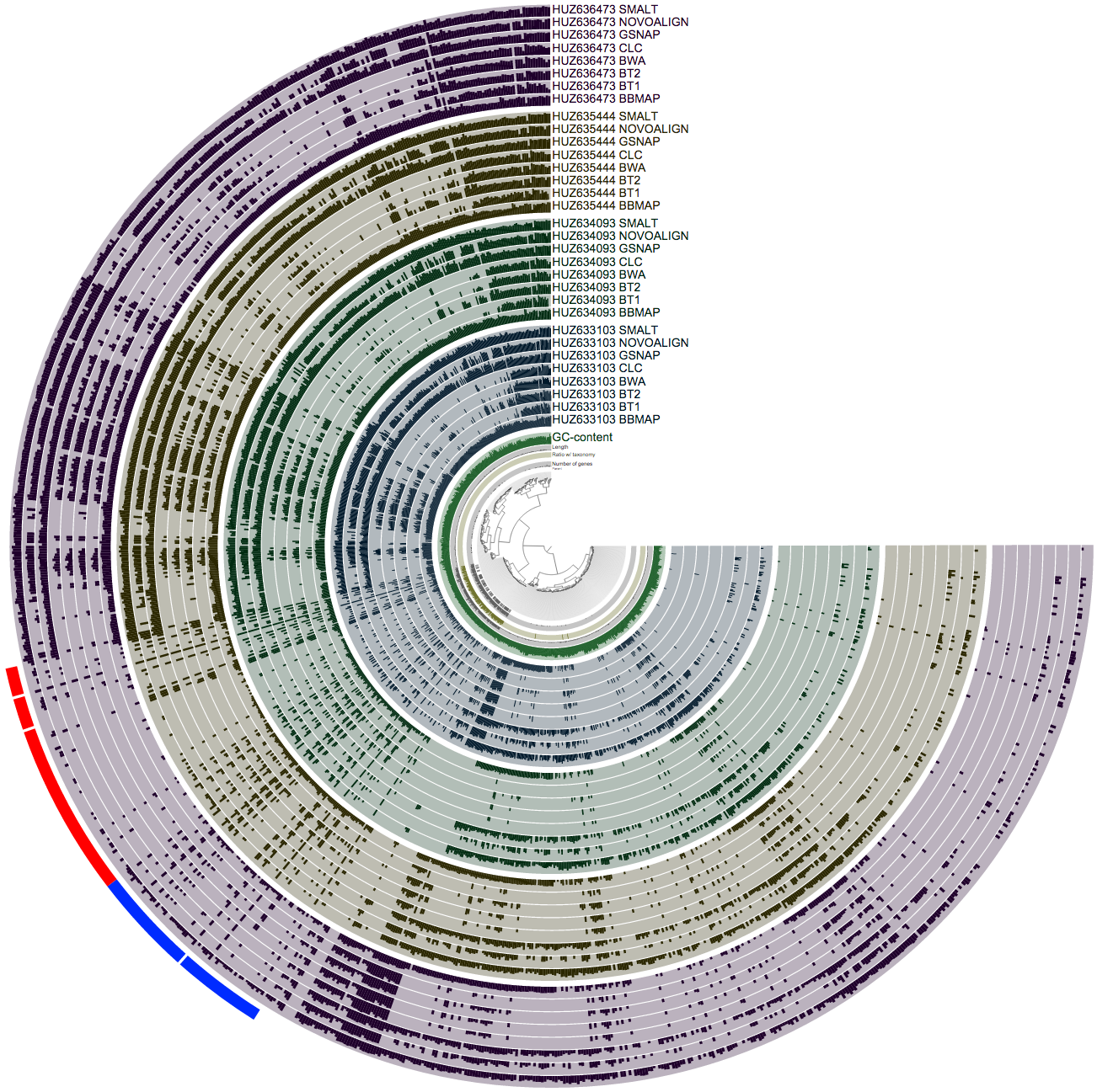
The previous view displayed the average number of reads mapped to each split. In contrast, in this one, each bar represents the number of SNPs identified in a given split. The amount of discrepancy is just mind blowing.
To better understand the coverage patterns, I zoomed to a random region of the tree with a lot of SNPs reported:
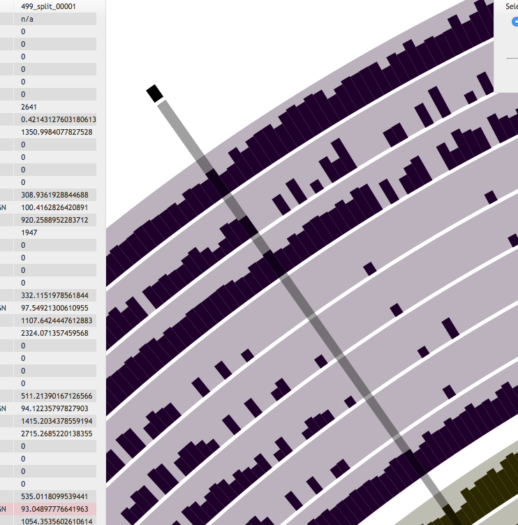
One of the right-click options is inspect, which we use very frequently. Here is the inspection of this particular split, and how short reads were mapped to it from individual mappers:
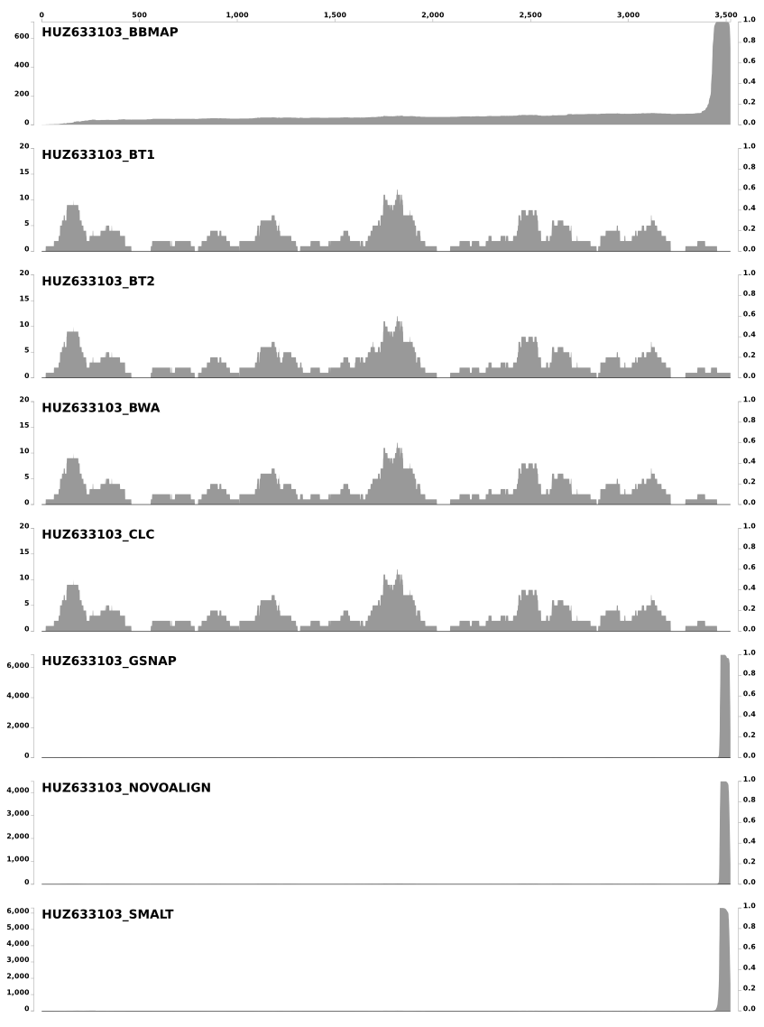
The Y-axes show the coverage values, and the X-axis shows the nucleotide position on the split. Because it was quite crazy for BBMAP, I removed SNP scores that are shown for each nucleotide position (they were so many of them that it was not possible to see the coverage of short reads). In this case CLC, BWA, Bowtie, and Bowtie2 is pretty much identical. In fact the coverage of short reads they mapped to this particular split is so identical that it gives a sense of trust that they definitely did a good job. On the other hand BBMAP, SMALT, GSNAP, and Novoalign mapped too many reads to this split than they should have, especially to the last 100-150nt part. Interestingly, BBMAP mapped reads to the entire length of the split with a steady increase in coverage (see the X-axis). Although in this particular case all of them map vast number of reads at the end of the contig, inspecting other splits gave me the impression that SMALT, GSNAP, and Novoalign always make similar mistakes (either they all over-map to the beginning, or to the end, or both ends of a split), and BBMAP most of the time does its own thing (and most of the time maps everything everywhere) with the default parameters.
Final words
It is almost certain that by optimizing parameters of BBMAP, SMALT, GSNAP, and Novoalign, it would have been possible to get them to a level where they produce comparable results to the other four. These results show that (1) one should be very careful with the default parameters when mapping metagenomic short reads to contigs, and (2), as Bing put very eloquently during one of our discussions, “the portion of reads that can be mapped is one factor, but not necessarily the most appropriate one”.
The parameter search for best mapping must be well-guided. Because the unsupervised genome binning approaches that pay attention to the coverage of contigs (i.e., CONCOCT, ESOMs, or GroupM), as well as the supervised ones, will benefit from accurate coverage estimates for contigs. This quick comparison also shows why it is crucial to go back and check mapping results very carefuly. I saw some irregular mapping results with Bowtie2 occasionally while inspecting splits, but it seems Bowtie, BWA and CLC overall did a good job with their default parameters for metagenomic mapping as the comparative analysis of this small -yet somewhat challenging- dataset suggests.
I thank Bing Ma for working with me on this. I also thank Jacques Ravel and Pawel Gajer for putting us in touch. contigs