Table of Contents
- Introduction
- Generating an anvi’o genomes storage
- Running a pangenome analysis
- Displaying the pan genome
- Inspecting gene clusters
- Inferring the homogeneity of gene clusters
- Concept of homogeneity
- Functional and geometric homogeneity estimates in anvi’o
- Using homogeneity indices in pangenomes
- Calculating rarefaction curves and Heaps’ Law parameters
- Splitting the pangenome
- Quantifying functional enrichment in a pangenome
- Computing the average nucleotide identity for genomes (and other genome similarity metrics too!)
- Summarizing an anvi’o pan genome
- Creating a pangenome with functions
The latest version of anvi’o is v7.1. See the release notes.
If you find a mistake on this page or would you like to update something in it, please feel free to edit its source by clicking the edit button at the top-right corner (which you will see if you are logged in to GitHub) 😇
With the anvi’o pangenomics workflow you can,
- Identify gene clusters across your genomes, by providing anvi’o with two or more FASTA files (and/or anvi’o contigs databases.
- Interactively visualize your pangenomes,
- Estimate relationships between your genomes based on gene clusters,
- Visualize rarefaction curves and calculate Heaps’ Law fit for your pangenomes,
- Interactively (or programmatically) partition gene clusters into bins,
- Perform phylogenomic analyses on-the-fly given a set of gene clusters,
- Annotate your genes, and inspect amino acid alignments within your gene clusters,
- Extend your pangenome with contextual information about your genomes or gene clusters,
- Quantify within-gene cluster statistics with geometric and biochemical homogeneity indices,
- Perform functional enrichment analyses on groups of genomes in your pangenome,
- Compute and visualize average nucleotide identity scores between you genomes, and more.
You can use anvi’o for pangenomic workflow even if you haven’t done any metagenomic work with anvi’o. All you need is an anvi’o installation, and a FASTA file for each of your genomes.
Introduction
The anvi’o pangenomic workflow described here will walk you through the following steps:
-
Generate an anvi’o genomes-storage-db using the program anvi-gen-genomes-storage.
-
Generate an anvi’o pan-db using the program anvi-pan-genome (which requires a genomes storage)
-
Display results in anvi’o interactive interface using the program anvi-display-pan.
You can then use the interactive interface to bin your gene clusters into collections, or use the program anvi-import-collection to import bins for your gene clusters, and finally you can use the program anvi-summarize to create a static HTML summary of your pangenome. Easy peasy!
The following sections will detail each step, and culminating in an example run will follow, but let’s first make sure you have all the required dependencies installed and your installation is good to go.
Dependencies
If your system is properly setup, this anvi-self-test command should run without any errors:
$ anvi-self-test --suite pangenomics
Generating an anvi’o genomes storage
A genomes storage is a special anvi’o database that stores information about genomes. A genomes storage can be generated only from external-genomes, only from internal-genomes, or a combination of both. Before we go any further, here are some definitions to clarify things:
-
An external genome is anything you have in a FASTA file format (i.e., a genome you have downloaded from NCBI, or obtained through any other way). Which means, you will need to convert each of your FASTA file into an anvi’o contigs database first using the program anvi-gen-contigs-database. Please read the contigs-db artifact to make sure you populate your contigs database with most useful information (such as annotating your genes with functions, and so on).
-
An internal genome is any genome bin you stored in an anvi’o collection (after binning and/or refining genomes from metagenomes in anvi’o). Working with internal genomes is quite straightforward since you already have an anvi’o contigs and an anvi’o profile database for them, but don’t worry if you are reading this tutorial and this does not yet make sense to you.
You can create a new anvi’o genomes storage using the program anvi-gen-genomes-storage, which will require you to provide descriptions of genomes to be included in this storage. File formats for external genome and internal genome descriptions differ slightly. For instance, this is an example --external-genomes file:
| name | contigs_db_path |
|---|---|
| Name_01 | /path/to/contigs-01.db |
| Name_02 | /path/to/contigs-02.db |
| Name_03 | /path/to/contigs-03.db |
| (…) | (…) |
and this is an example file for --internal-genomes:
| name | bin_id | collection_id | profile_db_path | contigs_db_path |
|---|---|---|---|---|
| Name_01 | Bin_id_01 | Collection_A | /path/to/profile.db | /path/to/contigs.db |
| Name_02 | Bin_id_02 | Collection_A | /path/to/profile.db | /path/to/contigs.db |
| Name_03 | Bin_id_03 | Collection_B | /path/to/another_profile.db | /path/to/another/contigs.db |
| (…) | (…) | (…) | (…) | (…) |
For names in the first column please use only letters, digits, and the underscore character.
Thanks to these two files, genomes described in anvi’o collections and genomes obtained via other sources can be combined and analyzed together seamlessly. The most essential need for the coherence within the genomes storage is to make sure each internal and external genome is generated identically with respect to how genes were called, how functions were assigned, etc. Anvi’o will check for most things, but it can’t stop you from doing mistakes. For instance, if the gene caller that identified open reading frames is not identical across all contigs databases, the genes described in genomes storage will not necessarily be comparable. If you are not sure about something, send us an e-mail, and we will be happy to try to clarify.
A real example for committed tutorial readers: A Prochlorococcus pangenome
For the sake of reproducibility, the rest of the tutorial will follow a real example.
We will simply create a pangenome of 31 Prochlorococcus isolate genomes that we used in this study.
If you wish to follow the tutorial on your computer, you can download the Prochlorococcus data pack (doi:10.6084/m9.figshare.6318833) which contains anvi’o contigs databases for these isolate genomes on your computer:
wget https://ndownloader.figshare.com/files/28834476 -O Prochlorococcus_31_genomes.tar.gz
tar -zxvf Prochlorococcus_31_genomes.tar.gz
cd Prochlorococcus_31_genomes
anvi-migrate *.db --migrate-dbs-safely
The directory contains anvi’o contigs databases, an external genomes file, and a TAB-delimited data file that contains additional information for each genome (which is optional, but you will see later why it is very useful). You can generate a genomes storage as described in this section the following way:
anvi-gen-genomes-storage -e external-genomes.txt \
                         -o PROCHLORO-GENOMES.db
Running a pangenome analysis
Once you have your genomes storage ready, you can use the program anvi-pan-genome to run the actual pangenomic analysis. This is the simplest form of this command:
$ anvi-pan-genome -g MY-GENOMES.db -n PROJECT_NAME
A real example for hardcore tutorial readers: A Prochlorococcus pangenome [continued]
Let’s run the pangenome using the genomes storage we created using the 31 Prochlorococcus isolates:
anvi-pan-genome -g PROCHLORO-GENOMES.db \
                --project-name "Prochlorococcus_Pan" \
                --output-dir PROCHLORO \
                --num-threads 6 \
                --minbit 0.5 \
                --mcl-inflation 10 \
                --use-ncbi-blast
Each parameter after the --project-name is optional (yet aligns to the way we run the pangenome for our publication).
The directory you have downloaded also contains a file called “layer-additional-data.txt”, which summarizes the clade to which each genome belongs. Once the pangenome is computed, we can add it into the pan database using the anvi’o program anvi-import-misc-data:
anvi-import-misc-data layer-additional-data.txt \
                      -p PROCHLORO/Prochlorococcus_Pan-PAN.db \
                      --target-data-table layers

New layers additional data...
===============================================
Data key "clade" .............................: Predicted type: str
Data key "light" .............................: Predicted type: str

New data added to the db for your layers .....: clade, light.
We all are looking for ways to enrich our pangenomic displays, and anvi’o’s additional data tables are excellent ways to do that. Please take a moment to learn more about them here.
When you run anvi-pan-genome, the program will,
-
Use all genomes in the genomes storage. If you would like to focus on a subset, you can use the parameter
--genome-names. -
Use only a single core by default. Depending on the number of genomes you are analyzing, this process can be very time consuming, hence you should consider increasing the number of threads to be used via the parameter
--num-threads. -
Use DIAMOND (Buchnfink et al., 2015) in ‘fast’ mode by default (or you can ask DIAMOND to be ‘sensitive’ by using the flag
--sensitive) to calculate the similarity of each amino acid sequence in every genome against every other amino acid sequence across all genomes (which clearly requires you to have DIAMOND installed). Alternatively you could use the flag--use-ncbi-blastto use NCBI’sblastpfor amino acid sequence similarity search. -
Use every gene call, whether they are complete or not. Although this is not a big concern for complete genomes, metagenome-assembled genomes (MAGs) will have many incomplete gene calls at the end and at the beginning of contigs. Our experiments so far suggest that they do not cause major issues, but if you want to exclude them, you can use the
--exclude-partial-gene-callsflag. -
Use the minbit heuristic that was originally implemented in ITEP (Benedict et al, 2014) to eliminate weak matches between two amino acid sequences. You see, the pangenomic workflow first identifies amino acid sequences that are somewhat similar by doing similarity searches, and then resolves gene clusters based on those similarities. In this scenario, weak similarities can connect gene clusters that should not be connected. Although the network partitioning algorithm can recover from these weak connections, it is always better to eliminate as much noise as possible at every step. So the minbit heuristic provides a mean to set a to eliminate weak matches between two amino acid sequences. We learned it from ITEP (Benedict MN et al, doi:10.1186/1471-2164-15-8), which is another comprehensive analysis workflow for pangenomes, and decided to use it because it makes a lot of sense. Briefly, If you have two amino acid sequences,
AandB, the minbit is defined asBITSCORE(A, B) / MIN(BITSCORE(A, A), BITSCORE(B, B)). So the minbit score between two sequences goes to1.0if they are very similar over the entire length of the ‘shorter’ amino acid sequence, and goes to0.0if (1) they match over a very short stretch compared even to the length of the shorter amino acid sequence or (2) the match between sequence identity is low. The default minbit is0.5, but you can change it using the parameter--minbit. -
Use the MCL algorithm (van Dongen and Abreu-Goodger, 2012) to identify clusters in amino acid sequence similarity search results. We use
2as the MCL inflation parameter by default. This parameter defines the sensitivity of the algorithm during the identification of the gene clusters. More sensitivity means more clusters, but of course more clusters does not mean better inference of evolutionary relationships. More information on this parameter and it’s effect on cluster granularity is here http://micans.org/mcl/man/mclfaq.html#faq7.2, but clearly, we, the metagenomics people will need to talk much more about this. So far in the Meren Lab we have been using2if we are comparing many distantly related genomes (i.e., genomes classify into different families or farther), and10if we are comparing very closely related genomes (i.e., ‘strains’ of the same ‘species’ (based whatever definition of these terms you fancy)). You can change it using the parameter--mcl-inflation. Please experiment yourself, and consider reporting! -
Utilize every gene cluster, even if they occur in only one genome in your analyses. Of course, the importance of singletons or doubletons will depend on the number of genomes in your analysis, or the question you have in mind. However, if you would like to define a cut-off, you can use the parameter
--min-occurrence, which is 1, by default. Increasing this cut-off will improve the clustering speed and make the visualization much more manageable, but again, this parameter should be considered in the context of each study. -
Use
euclideandistance andwardlinkage to organize gene clusters and genomes. You can change those using--distanceand--linkageparameters. -
Try to utilize previous search results if there is already a directory. This way you can play with the
--minbit,--mcl-inflation, or--min-occurrenceparameters without having to re-do the amino acid sequence search to gain time. If you are having hard time making anvi’o use the existing output files, please see the explanation in this issue. If you are not interested in using the previous search results, you can remove the output directory, or use the--overwrite-output-destinationsflag to redo the search from scratch.
You need another parameter? Well, of course you do! Let us know, and let’s have a discussion. We love parameters.
Once you are done, a new directory with your analysis results will appear. You can add or remove additional data items into your pan profile database using anvi’o additional data tables subsystem.
Displaying the pan genome
Once your analysis is done, you will use the program anvi-display-pan to display your results.
This is the simplest form of this command:
$ anvi-display-pan -p PROJECT-PAN.db -g PROJECT-PAN-GENOMES.db
The program anvi-display-pan is very similar to the program anvi-interactive, and the interface that will welcome you is nothing but the standard anvi’o interactive interface with slight adjustments for pangenomic analyses. Of course anvi-display-pan will allow you to set the IP address and port number to serve, add additional view data, additional layers, and/or additional trees, and more. Please familiarize yourself with it by running anvi-display-pan -h in your terminal.
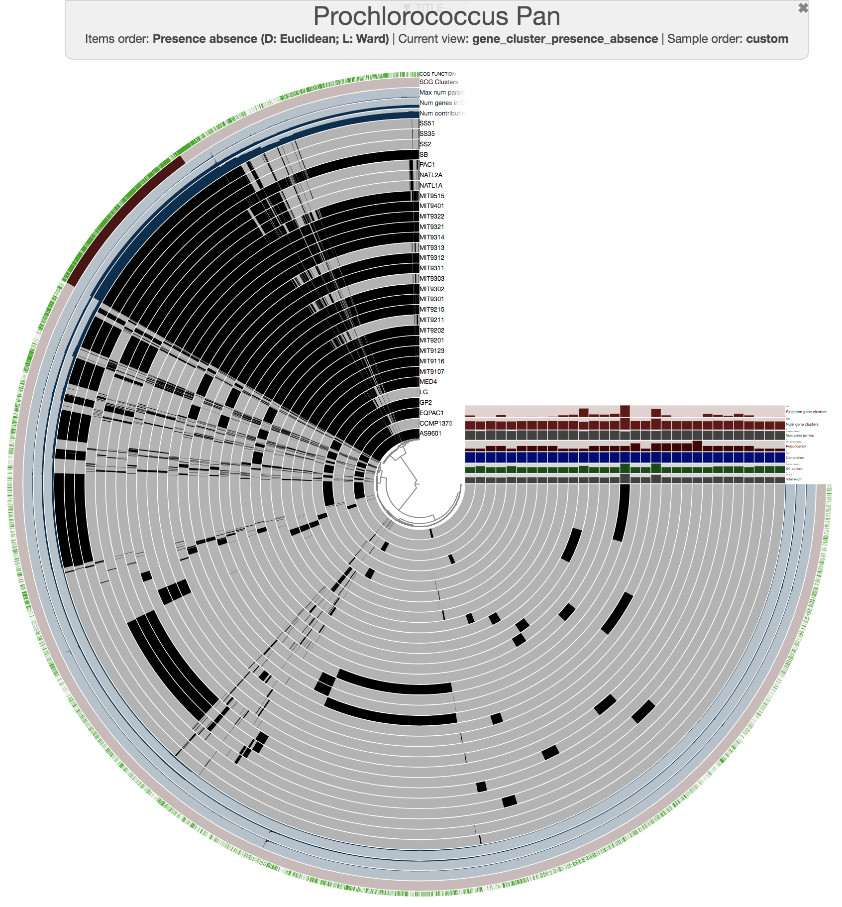
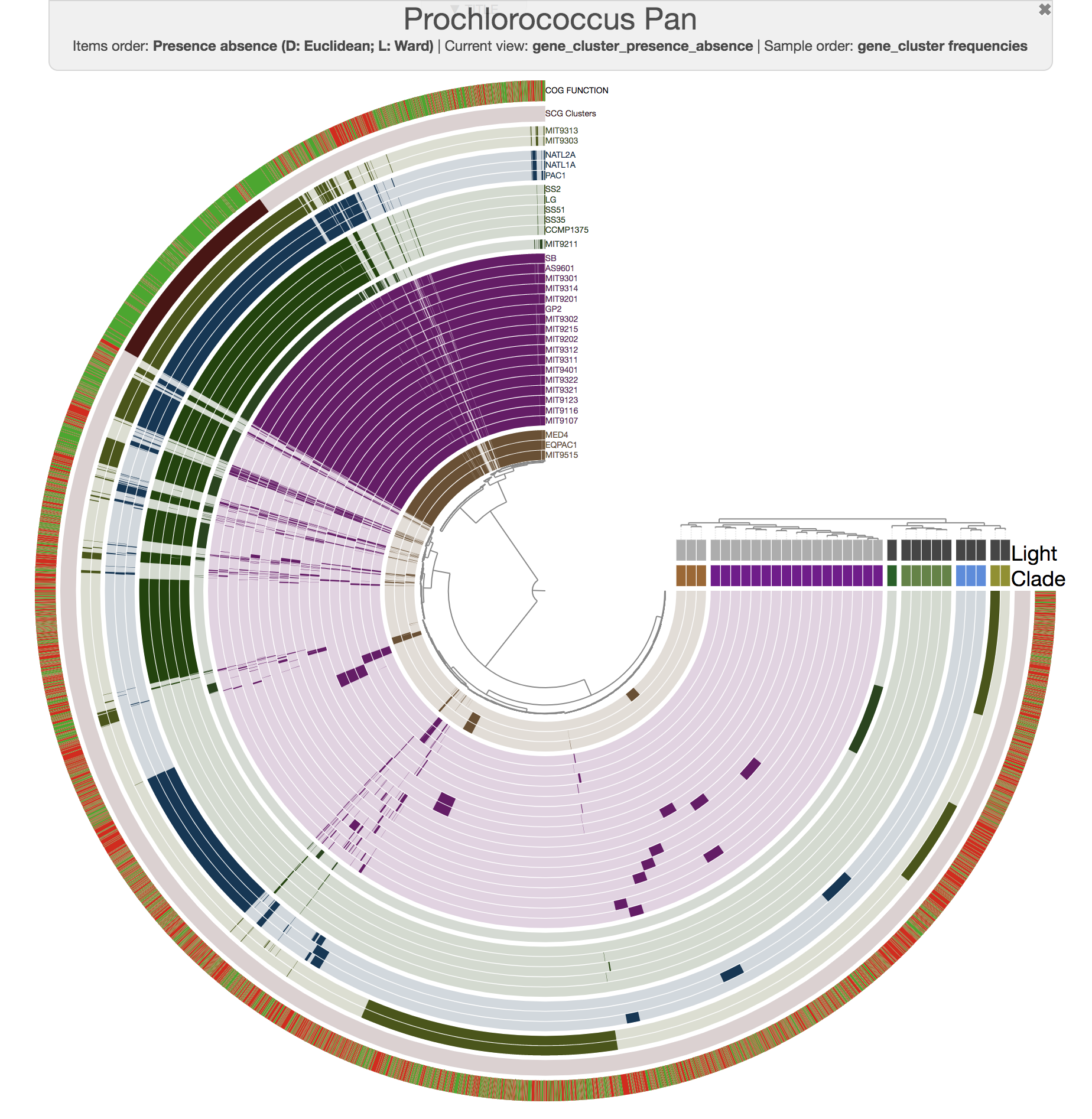
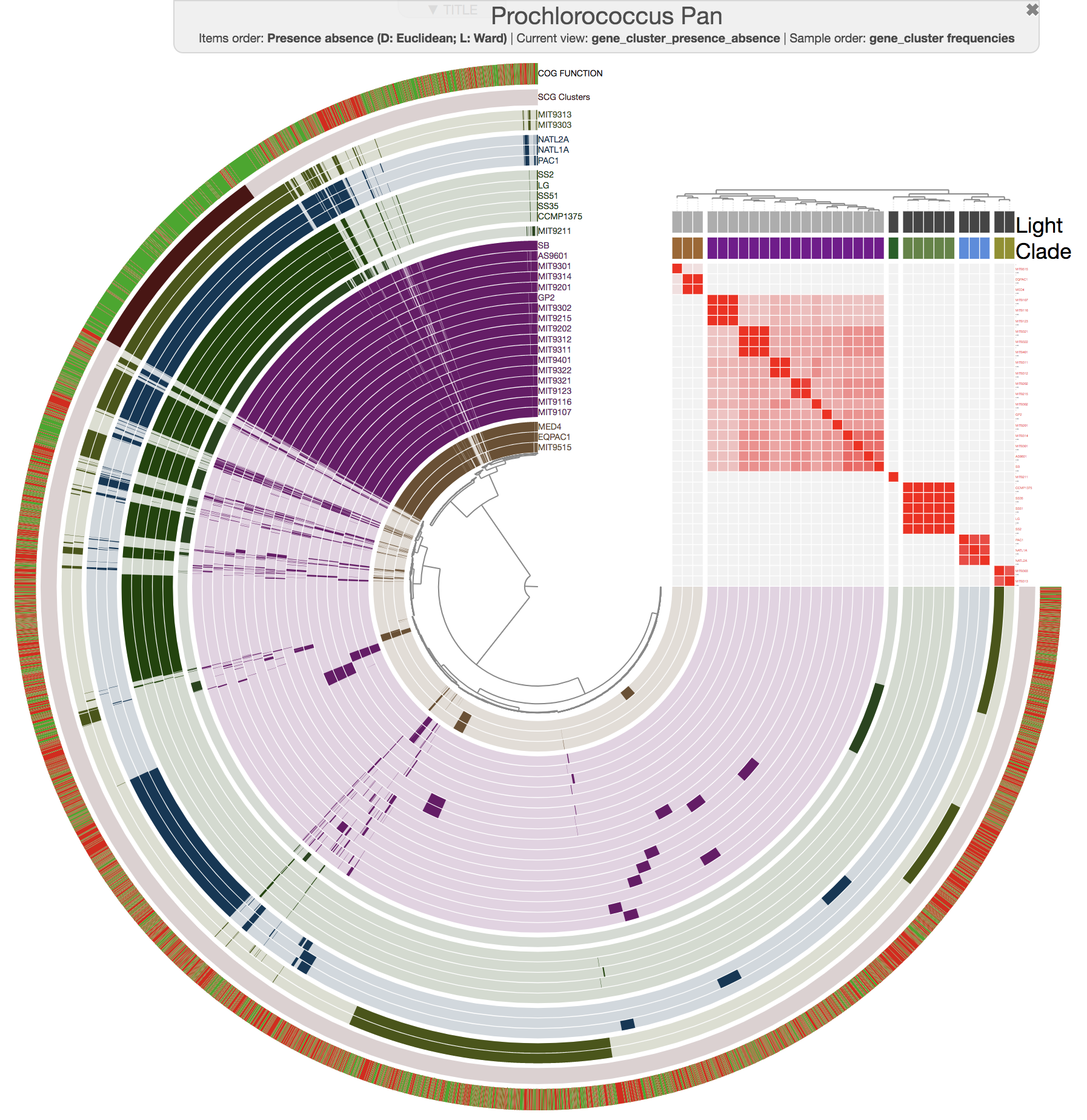
Here is the pangenome for the 31 Prochlorococcus isolate genomes we have created in the previous sections of this tutorial:
anvi-display-pan -g PROCHLORO-GENOMES.db \
                 -p PROCHLORO/Prochlorococcus_Pan-PAN.db
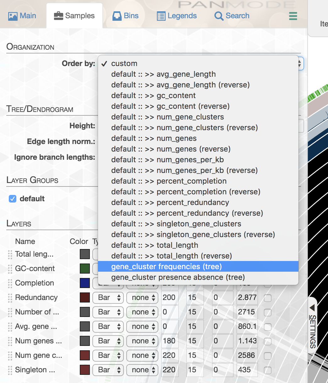
Looks ugly. But that’s OK (for now). For instance, to improve things a little, you may like to organize your genomes based on gene clustering results by selecting the ‘gene_cluster frequencies’ tree from the Samples Tab > Sample Order menu:
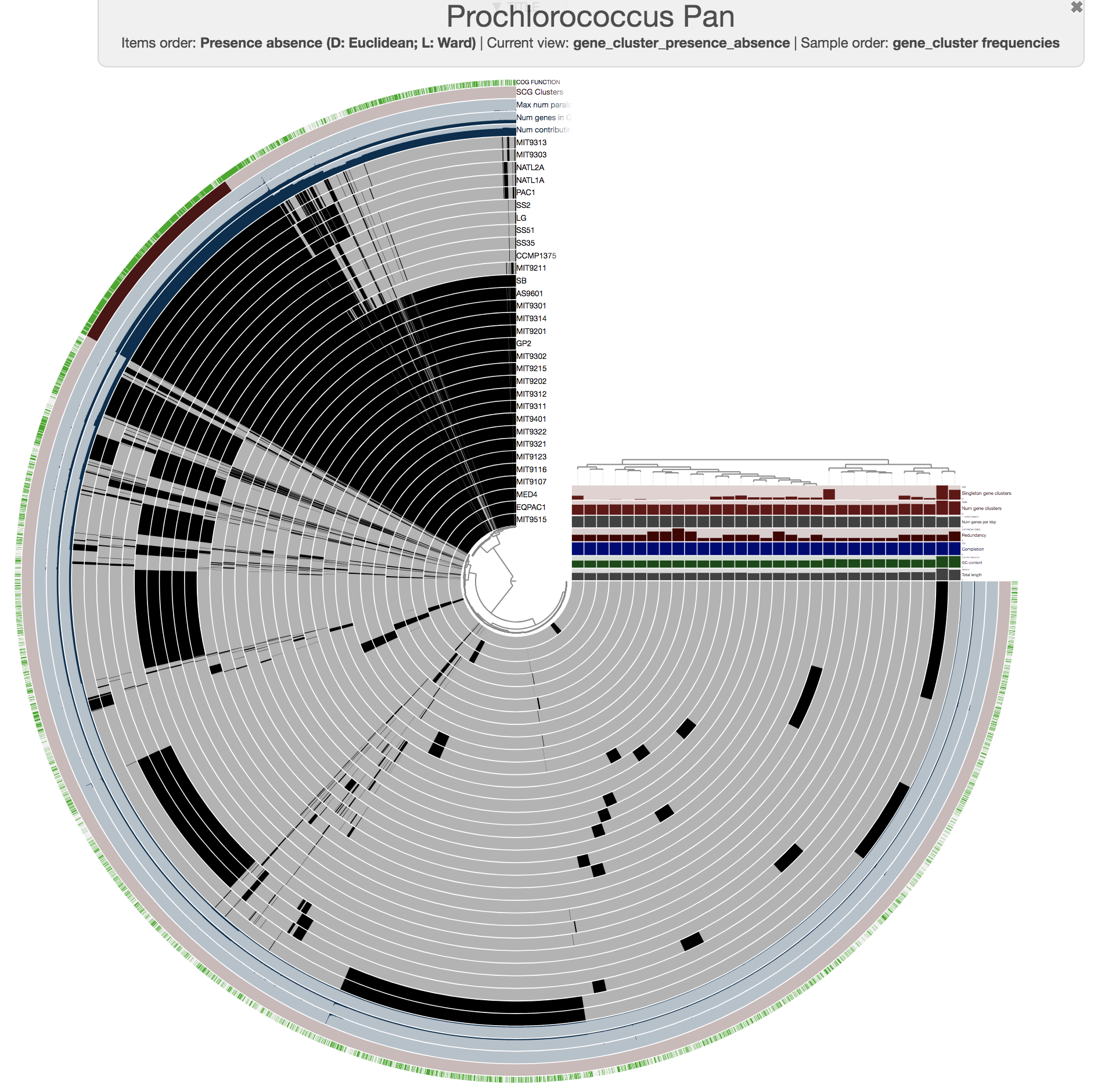
This is what happens when you draw it again (note the tree that appears on the right):
Looks more meaningful .. but still ugly.
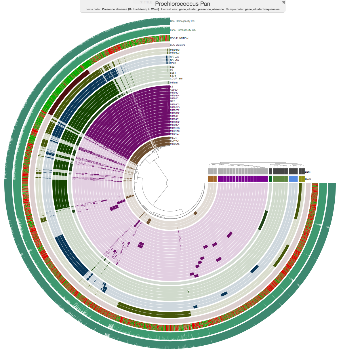
Well, this is exactly where you need to start using the interface more efficiently. For instance, this is the same pangenome after some changes using the additional settings items in the settings panel of the interactive interface:
If you downloaded the Prochlorococcus data pack, you will also find an anvi’o state file that you can import into your pan database using the program anvi-import-state:
anvi-import-state -p PROCHLORO/Prochlorococcus_Pan-PAN.db \
                  --state pan-state.json \
                  --name default
No excuses for bad looking pangenomes.
For an example, step-by-step instructions on how to improve a pangenome, see the polishing the pangenome section in this reproducible workflow.
Inspecting gene clusters
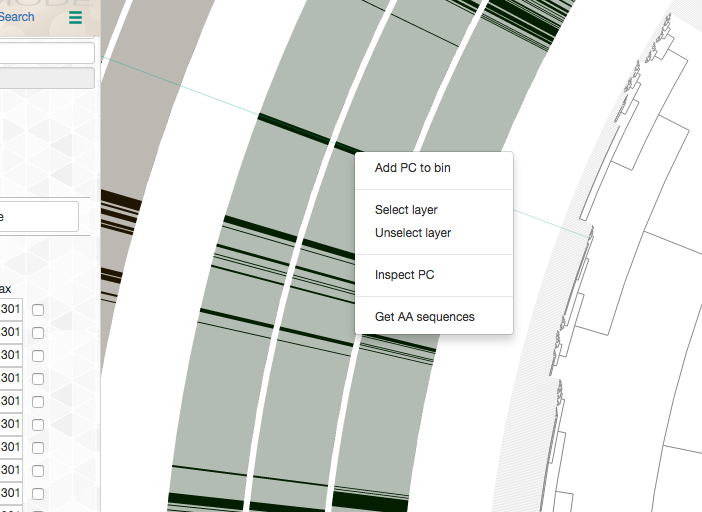
Every gene cluster in your analysis will contain one or more amino acid sequence that originate from one or more genomes. While there will likely be a ‘core’ section, in which all gene cluster will appear in every genome, it is also common to find gene clusters that contain more than one gene call from a single genome (i.e., all multi-copy genes in a given genome will end up in the same gene cluster). Sooner or later you will start getting curious about some of the gene clusters, and want to learn more about them. Luckily you can right-click on to any gene cluster, and you would see this menu (or maybe even more depending on when you are reading this article):
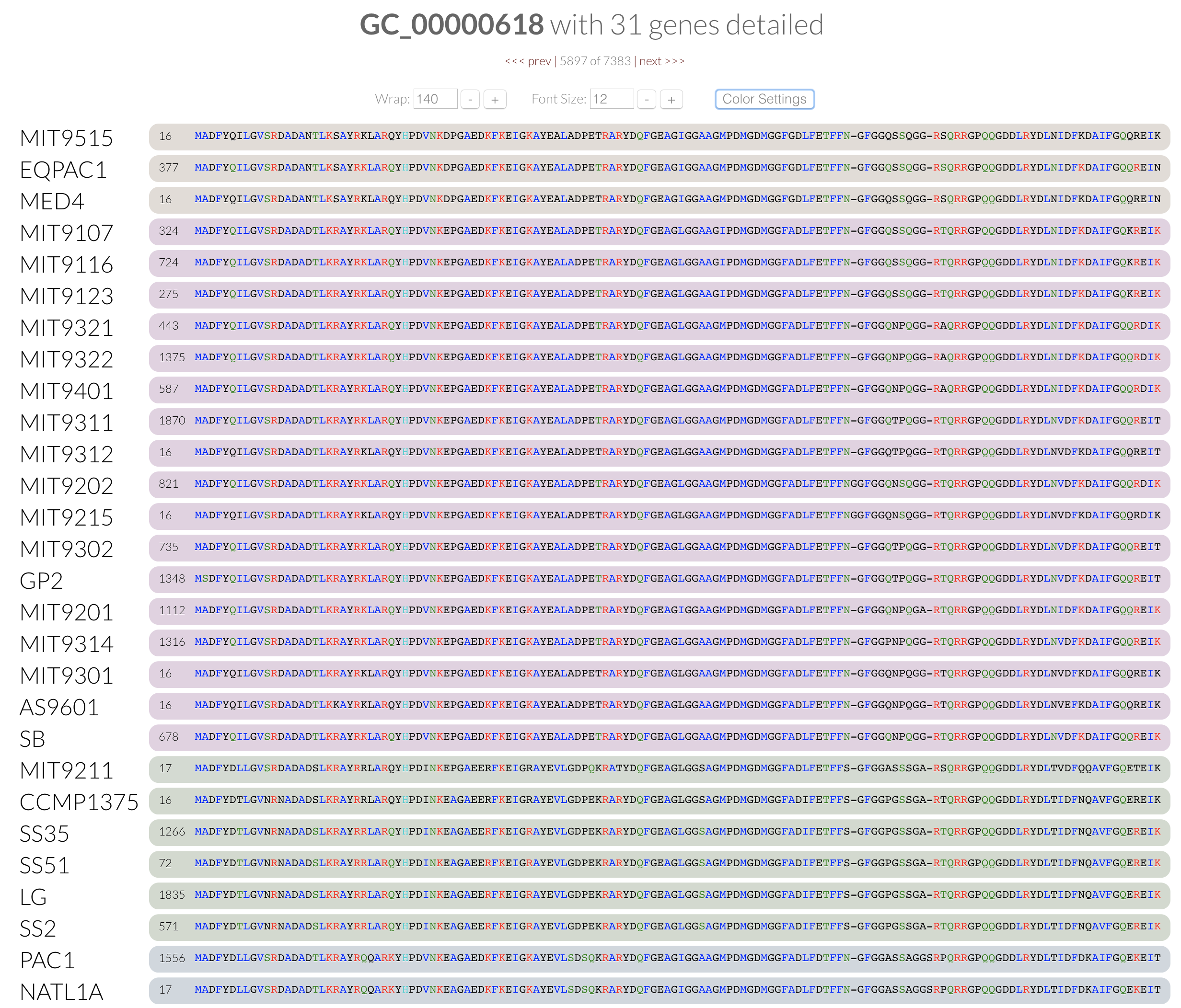
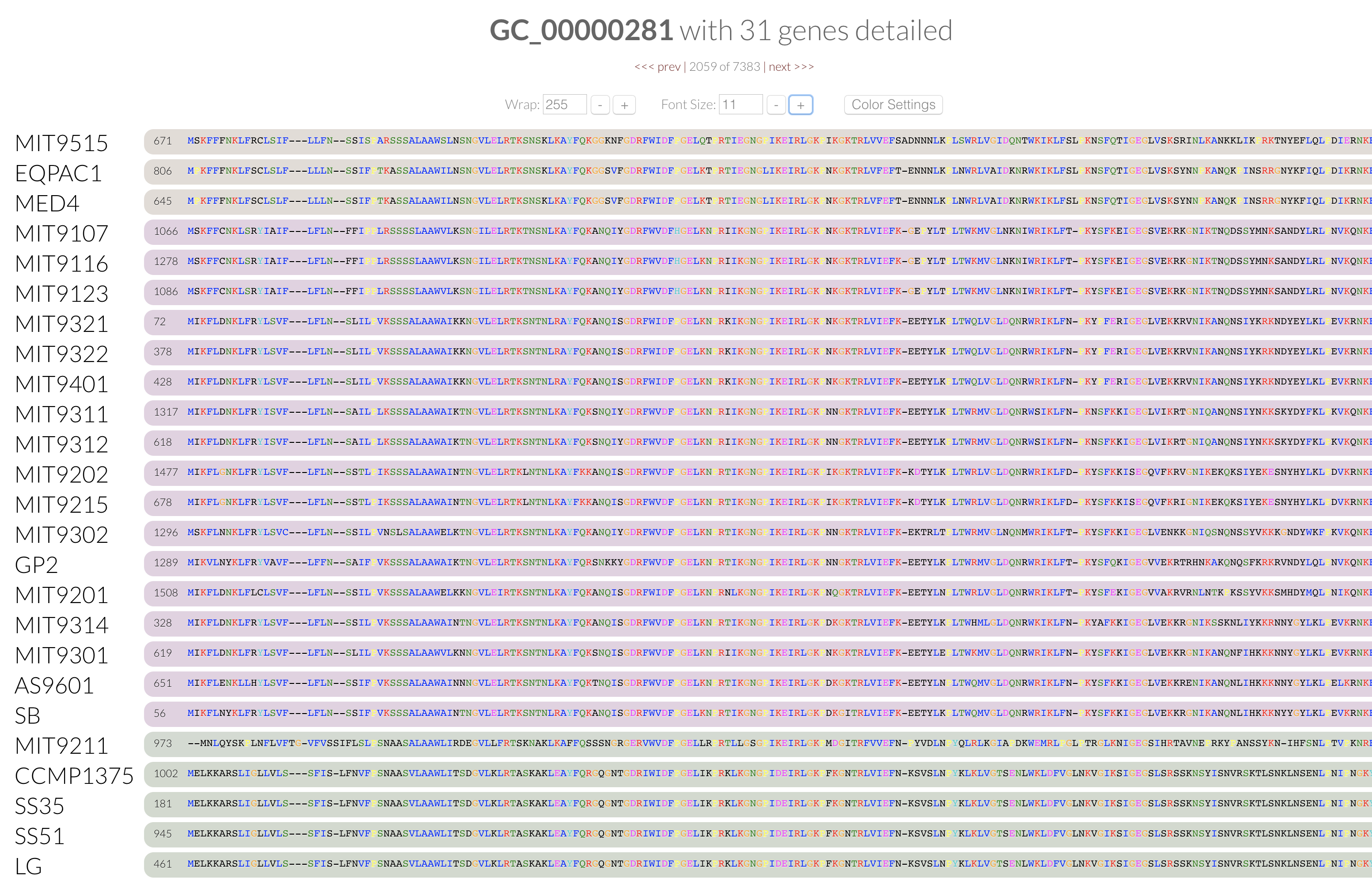
For instance, if you click ‘Inspect gene cluster’, you will see all the amino acid sequences from each genome that went into that gene cluster (with the same order and background colors of genomes as they are arranged in the main display):
You can learn more about the amino acid color coding algorithm here.
It is not only fun but also very educational to go through gene clusters one by one. Fine. But what do you do if you want to make sense of large selections?
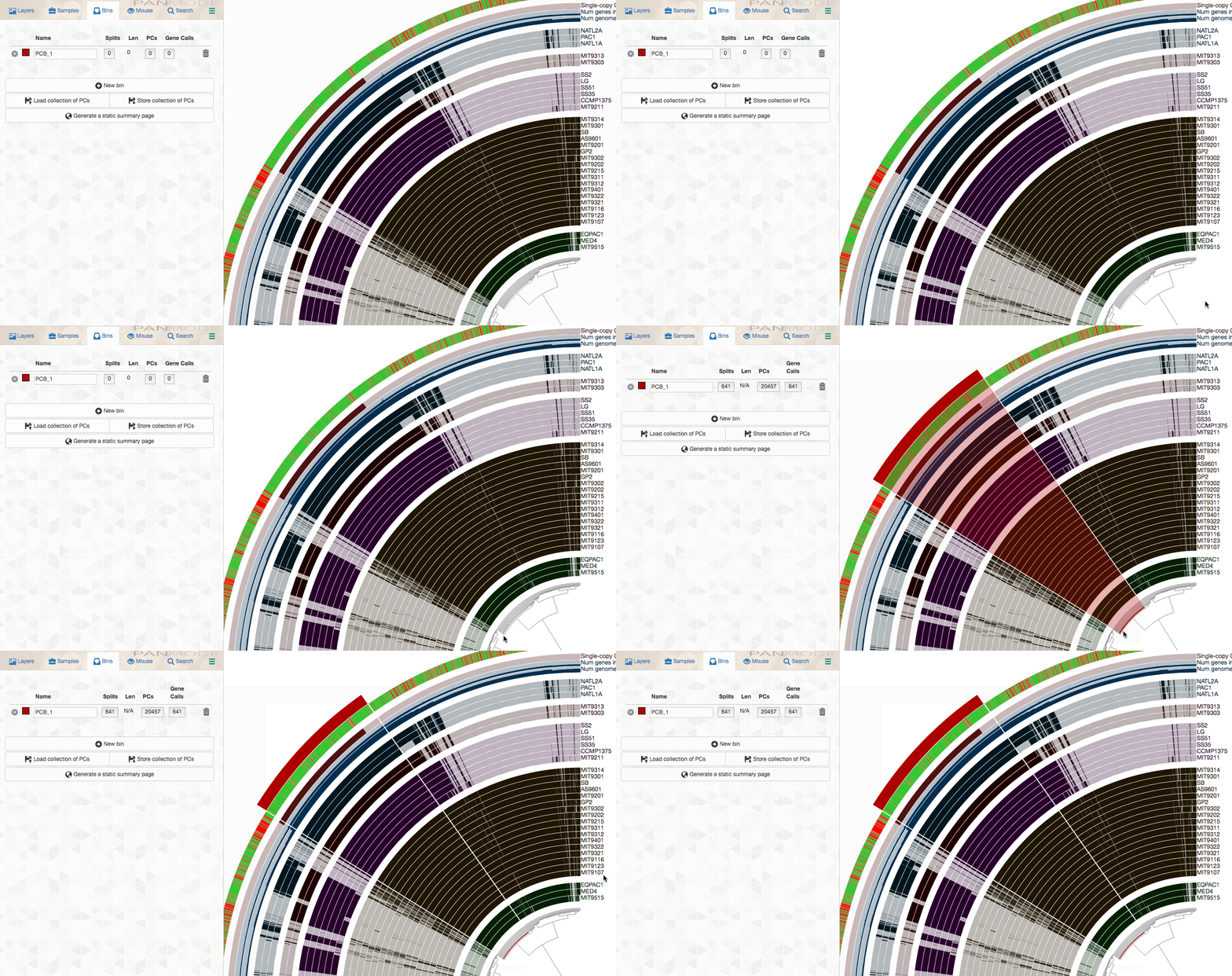
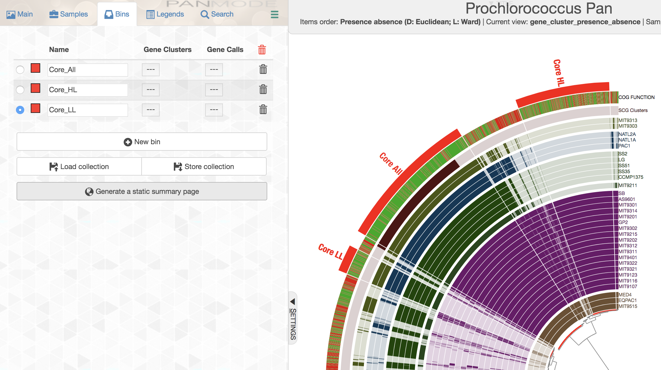
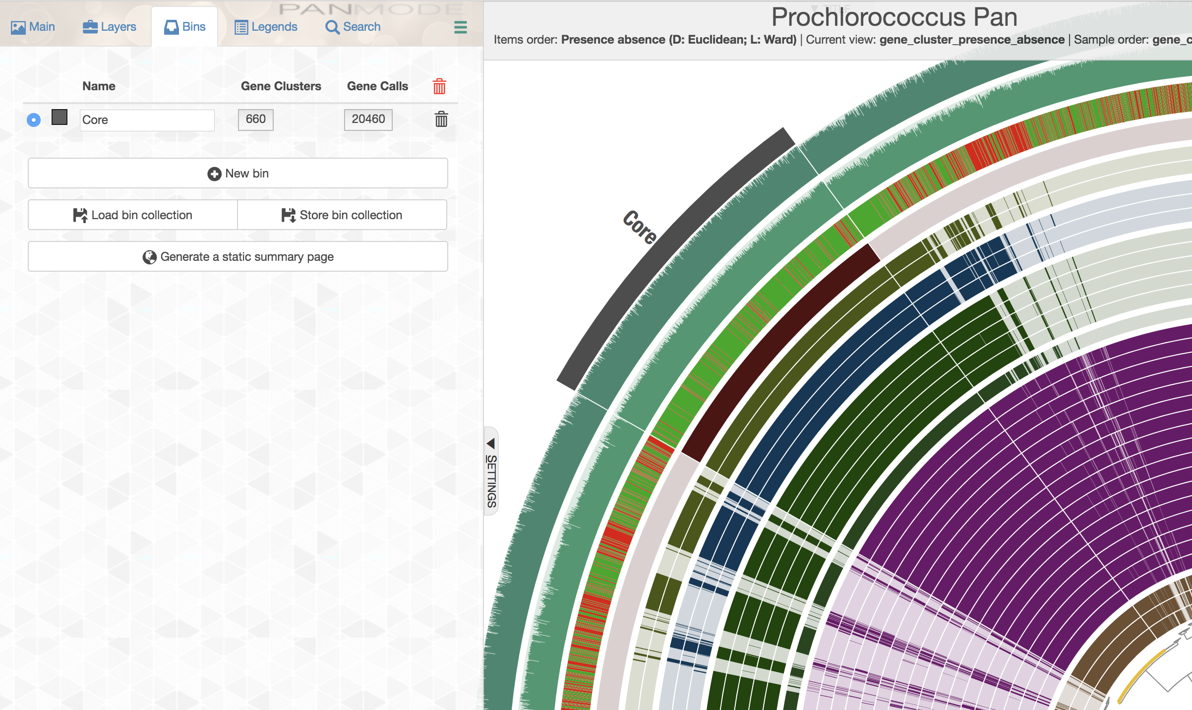
As you already know, the anvi’o interactive interface allows you to make selections from the tree. So you can select groups of gene clusters into bins (don’t mind the numbers on the left panel, there clearly is a bug, and will be fixed in your version):
You can create multiple bins with multiple selections, and even give them meaningful names if you fancy:
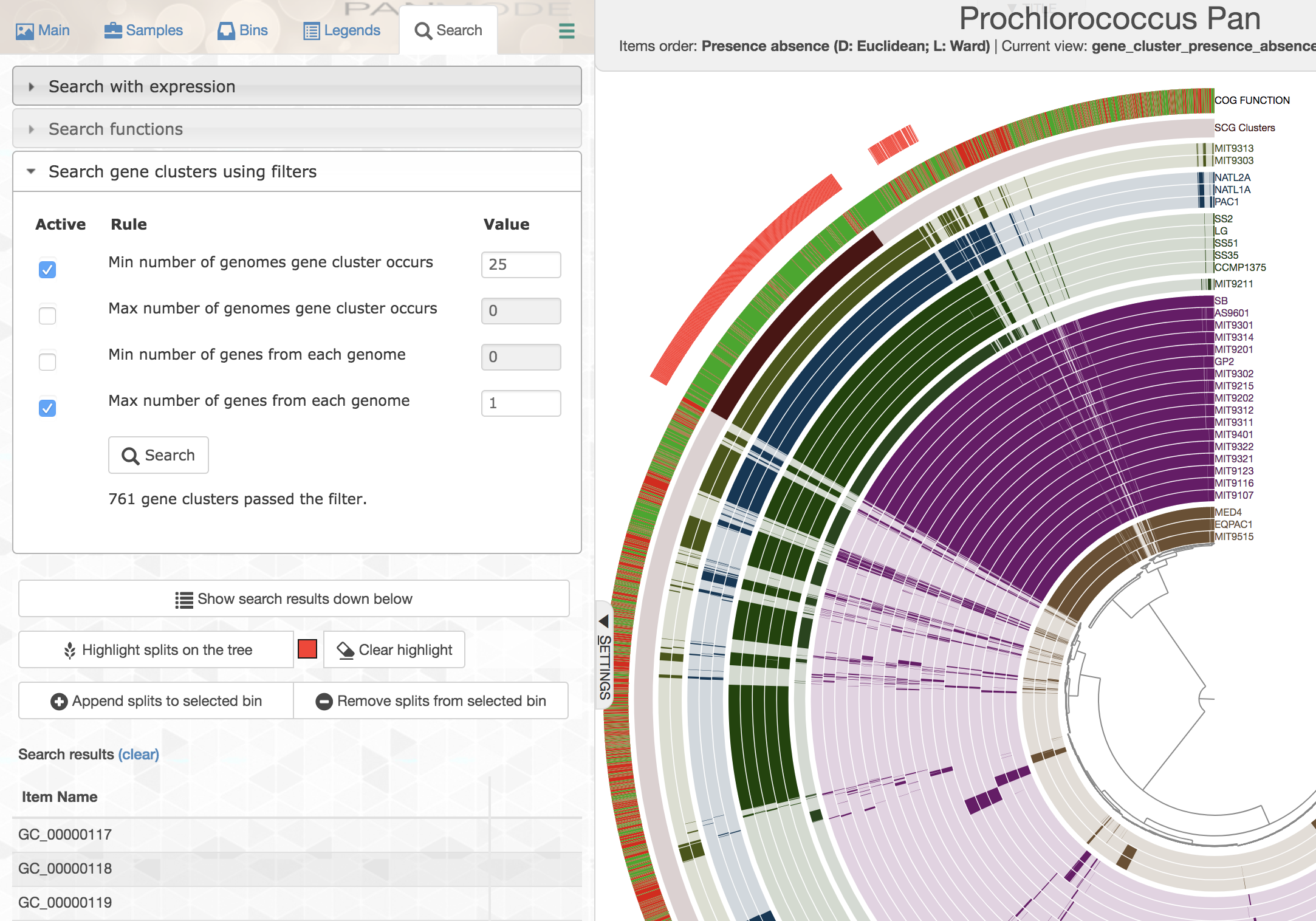
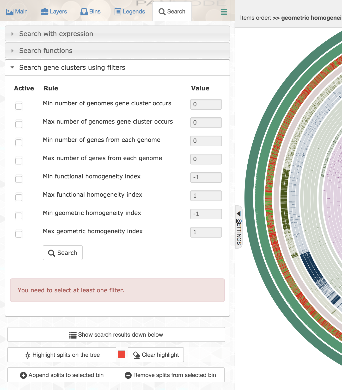
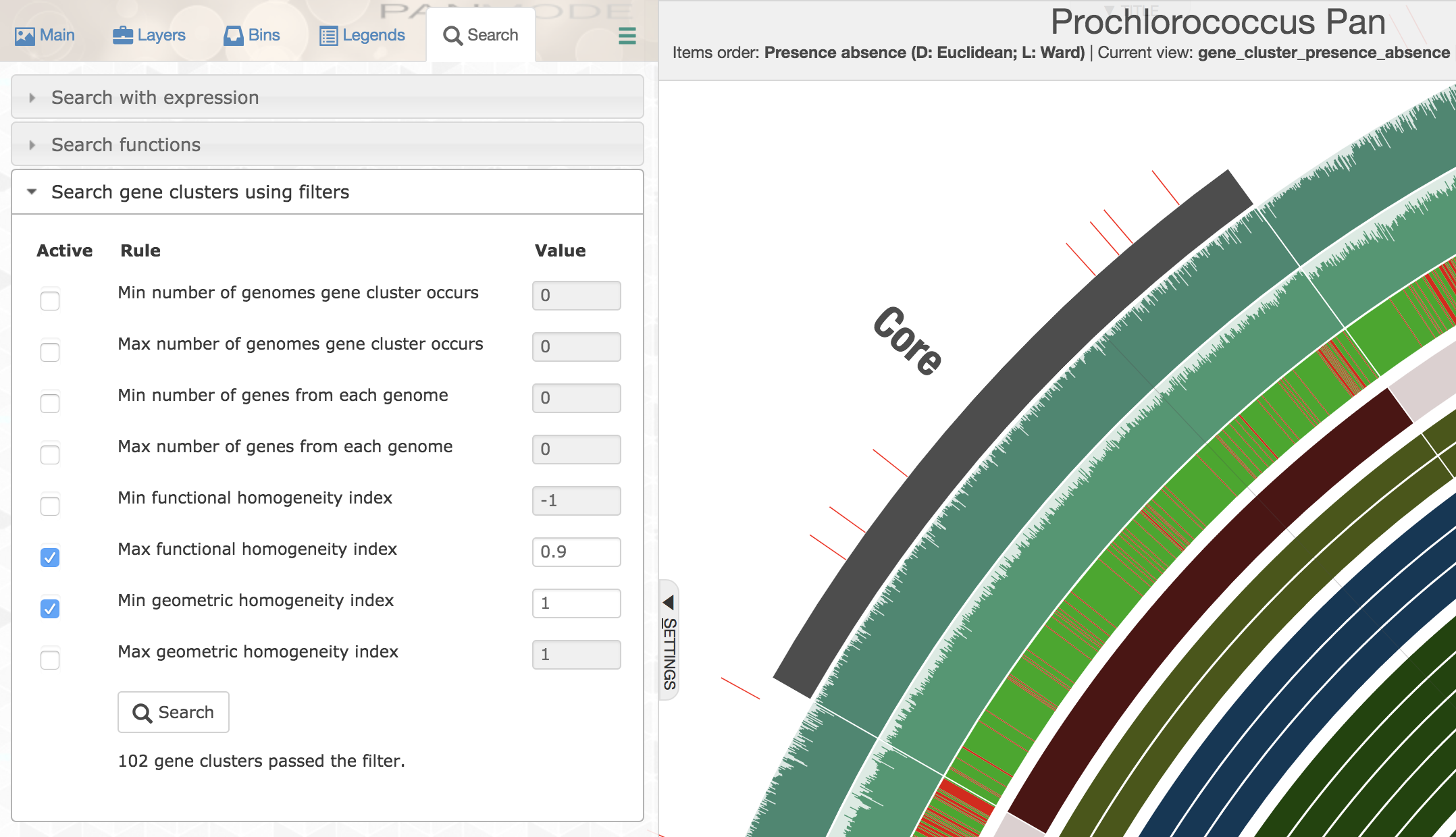
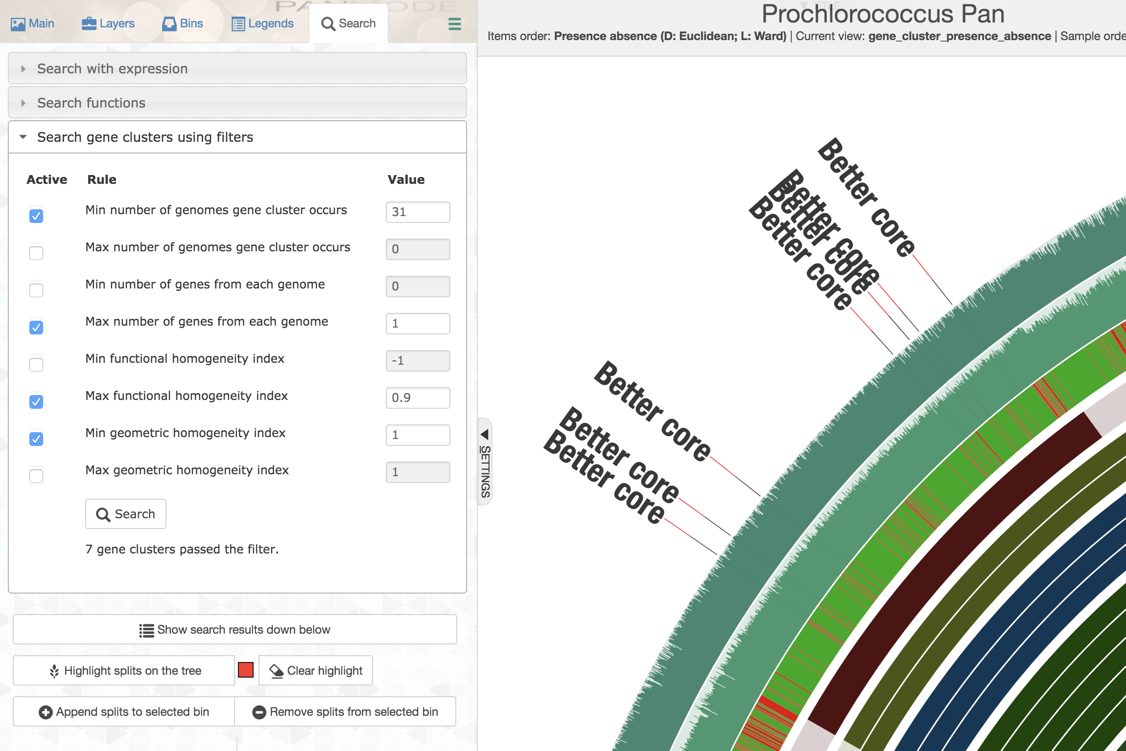
While selecting gene clusters manually using the dendrogram is an option, it is also possible to identify them using the search interface that allows you to define very specific search criteria:
You can highlight these selections in the interface, or you can add them to a collection to summarize them later.
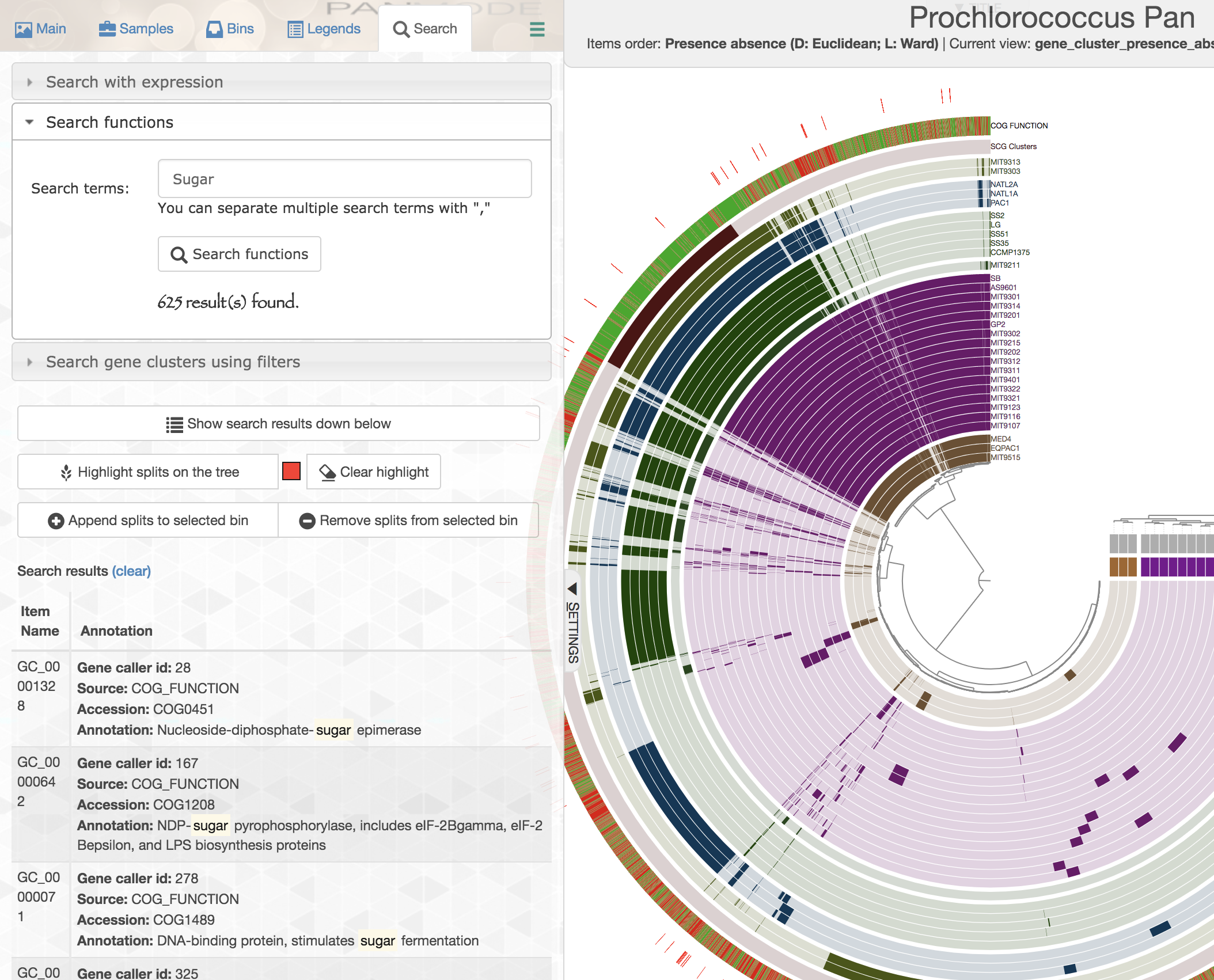
In addition, you can search gene clusters also based on functions:
Similarly, you can add these gene clusters into collections with whatever name you like, and summarize those collections later.
Advanced access to gene clusters is also possible through the command line through the program anvi-get-sequences-for-gene-clusters. For more information see this issue or this vignette.
Inferring the homogeneity of gene clusters
This functionality is available since anvi’o v5.2 thanks to the efforts of Mahmoud Yousef.
Gene clusters are good, but not all gene clusters are created equal. By simply inspecting the alignments within just a few of gene clusters, you can witness differing levels of disagreements between amino acid sequences across different genomes.
Concept of homogeneity
A gene cluster may contain amino acid sequences from different genomes that are almost identical, which would be a highly homogeneous gene cluster. Another gene cluster may contain highly divergent amino acid sequences from different genomes, which would then be a highly non-homogeneous one, and so on.
One could infer the nature of sequence homogeneity within a gene cluster by focusing on two primary attributes of sequence alignments: functional homogeneity (i.e., how conserved aligned amino acid residues across genes), and geometric homogeneity (i.e., how does the gap / residue distribution look like within a gene cluster regardless of the identity of amino acids). While it is rather straightforward to have an idea about the homogeneity of gene clusters through the manual inspection of the aligned sequences within them, it has not been possible to quantify this information automatically. But anvi’o now has you covered.
Indeed, understanding the within gene cluster homogeneity could yield detailed ecological or evolutionary insights regarding the forces that shape the genomic context across closely related taxa, or help scrutinize gene clusters further for downstream analyses manually or programmatically. The purpose of this section is to show you how we solved this problem in anvi’o and to demonstrate its efficacy.
Functional and geometric homogeneity estimates in anvi’o
Anvi’o pangenomes contains two layers that summarize homogeneity indices for each gene cluster (and an additional one that combines the two).
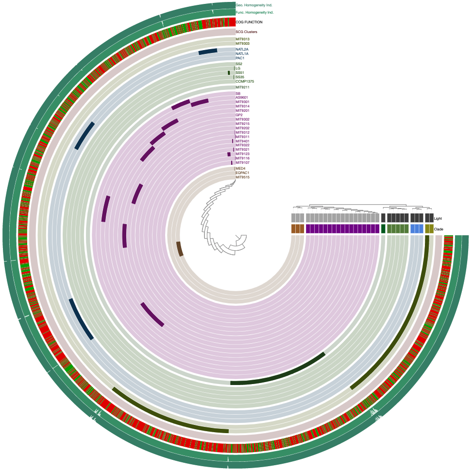
Here is an example in the context of our Prochlorococcus pangenome (see the outermost two additional layers):
Homogeneity indices are calculated based on the alignment. If the alignment for some reason fails for a given set of genes in a gene cluster, the homogeneity indices for it will show -1.
Geometric homogeneity index
The geometric homogeneity index indicates the degree of geometric configuration between the genes of a gene cluster. Specifically, we look for the gap/residue patterns of the gene cluster that have been determined by the alignment. The alignment process by definition aligns similar sections of genes to each other, and denotes missing residues (or different structural configurations of gene contexts) through gap characters. If gap/residue distribution patterns are mostly uniform throughout the gene cluster, then this gene cluster will have a high geometric homogeneity, and the maximum value of 1.0 indicates that are no gaps in the alignment.
Anvi’o computes the geometric homogeneity index by combining analysis of the gene cluster content in two levels: the site-level analyses (i.e., vertically aligned positions) and the gene-level analyses (i.e., horizontally aligned positions because they are in the same gene). We convert the information in a gene cluster into a binary matrix, where gaps and residues are simply represented by 1s and 0s, and we utilize the logical operator xor to identify and enumerate all comparisons that have a different pattern. In site-level homogeneity checks, the algorithm sweeps from left to right and identifies these differences across aligned columns. In gene-level homogeneity checks, the algorithm sweeps from one gene to the next and identifies all differences in a gene where the pattern is not the same, effectively checking for the spread of gaps across the gene cluster. It is possible to skip the gene-level geometric homogeneity caluclations with the flag --quick-homogeneity. While this will not be as accurate or as comprehensive as the default approach, it may save you some time, depending on the number of genomes with which you are working.
Functional homogeneity index
In contrast, the functional homogeneity index considers aligned residues (by ignoring gaps), and attempts to quantify differences across residues in a site by considering the biochemical properties of differing residues (which could affect the functional conservation of genes at the protein-level). To do this, we divided amino acids into seven different “conserved groups” based on their biochemical properties. These groups are: nonpolar, aromatic, polar uncharged, both polar and nonpolar characteristics (these amino acids also lie in groups besides this one), acidic, basic, and mostly nonpolar (but contain some polar characteristics) (for more information please see this article). Then, the algorithm goes through the entire gene cluster and assigns a similarity score between 0 and 3 to every pair of amino acids at the same position across genes based on how close the biochemical properties of the amino acid residues are to each other. The sum of all assigned similarity scores is indicative of the functional homogeneity index of the gene cluster, and will reach to its maximum value of 1.0 if all residues are identical.
Both indices are on a scale of 0 to 1, where 1 is completely homogeneous and 0 is completely heterogeneous. If the algorithm is interrupted by a runtime error (due to unexpected issues such as not all genes being the same length for whatever reason, etc.), it will default to error values of -1 for the indices. So if you see a -1 in your summary outputs, it means we failed to make sense of the alignments in that gene cluster for some reason :/
In reality, the complex processes that influence protein folding and the intricate chemical interactions between amino acid residues should remind us that these assessments of similarity are only mere numerical suggestions, and do not necessarily reflect accurate biochemical insights, which is not the goal of these homogeneity indices.
Using homogeneity indices in pangenomes
Given all of that, let’s look at our pangenome again. What are they good for? Well, there is a lot one could do with these homogeneity indices, and it would be unfair to expect this tutorial to cover all of them. Nevertheless, here is an attempt to highlight some aspects of it.
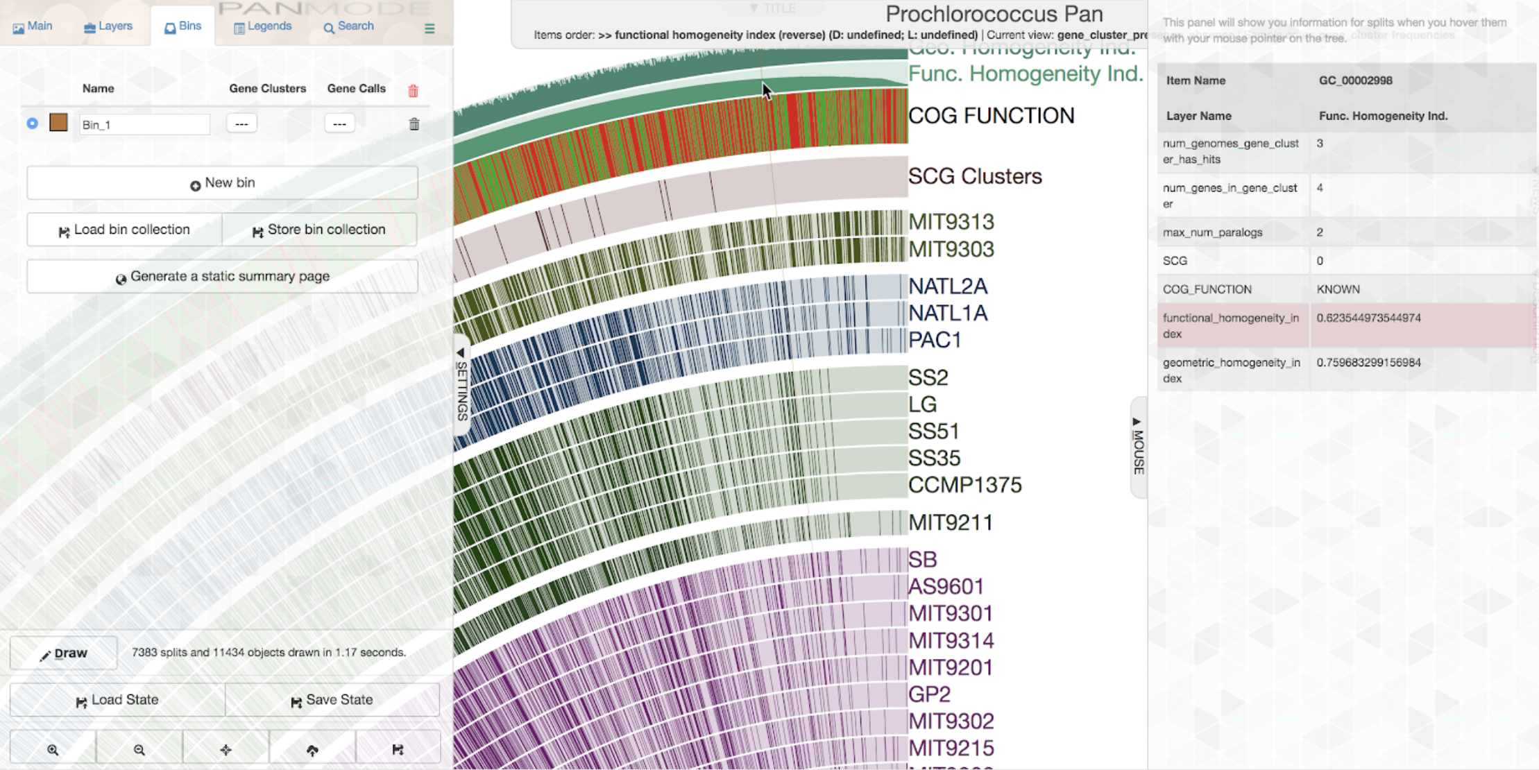
To get a quick idea about some of the least homogeneous gene clusters, one could order gene clusetrs based on increasing or decreasing homogeneity. Let’s say we want to order it by increasing functional homogeneity (as you likely know already, this can be done through the “Items order” combo box in the main settings panel):
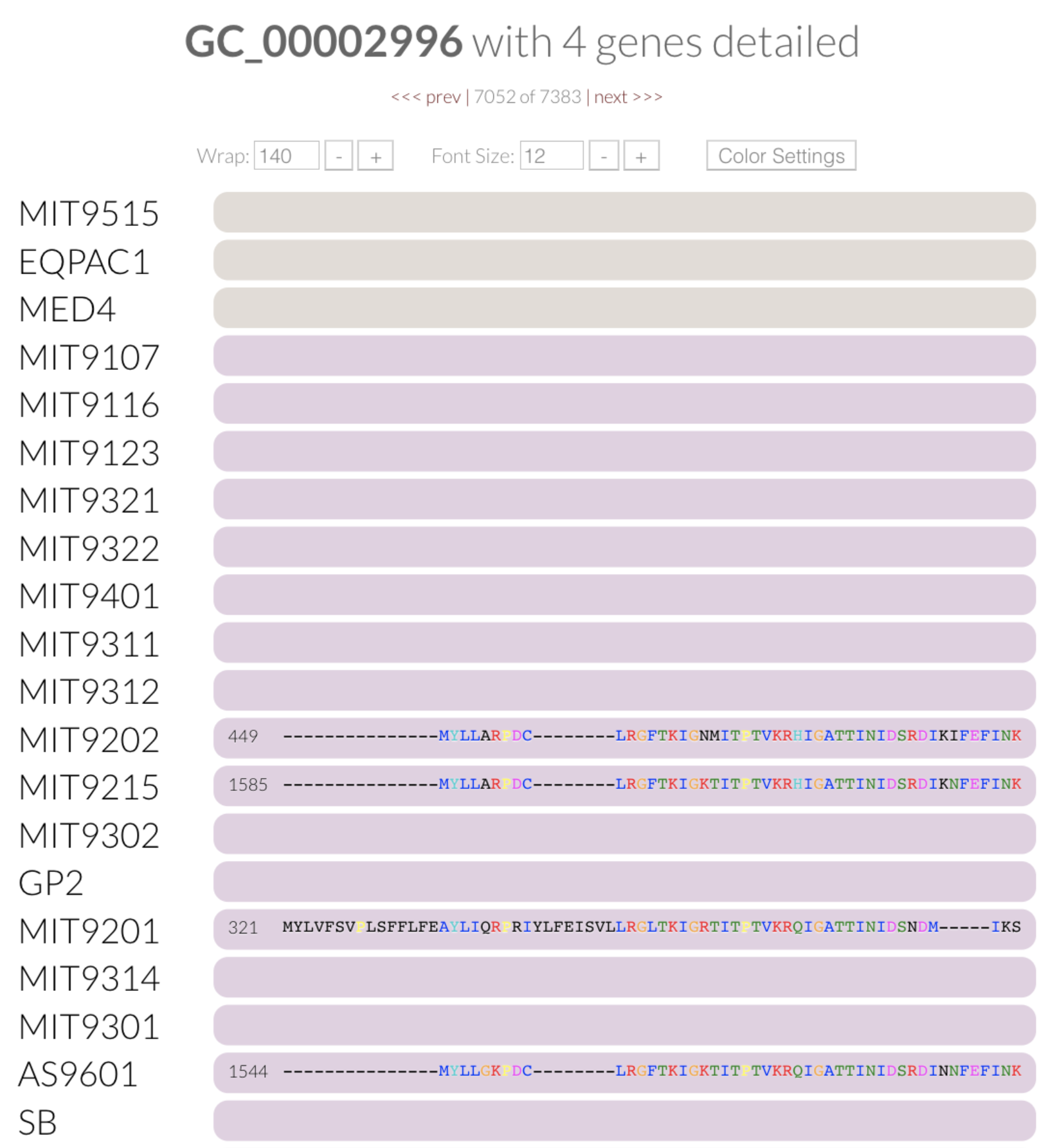
If you open the “Mouse” panel on the right side of your display, you can actually hover over the layer and see the exact value of the index for all gene clusters. The gene cluster shown underneath the cursor in the figure above has a relatively low functional homogeneity estimate, but a higher geometric homogeneity. We can inspect the gene cluster to take a look for ourselves:
You can see why the relatively higher geometric homogeneity score makes sense. Three of these genes have the same gap/residue pattern, and the gaps at the end of the other gene throw things off slightly, making the geometric score close to 0.75. On the other hand, the color coding of the aligned amino acids also gives us a hint regarding the lack of functional homogeneity across them. We can do the same for the geometric homogeneity index. Try it yourself: order the pangenome based on the geometric homogeneity index, and inspect a gene cluster with a relatively low score.
So, what can we do for more in depth analyses of our gene clusters?
Anvi’o offers quite a powerful way to filter gene clusters both through the command line program anvi-get-sequences-for-gene-clusters, and through the interface for interactive exploration of the data:
Exploratory analyses
Let’s assume you wish to find a gene cluster that represents a single-copy core gene with very high discrepancy between its geometric homogeneity versus its functional homogeneity. As in, you want something that is highly conserved across all genomes, it is under structural constraints that keeps its alignment homogeneous, but it has lots of room to diversify in a way that impacts its functional heterogeneity. You want a lot. But could anvi’o deliver?
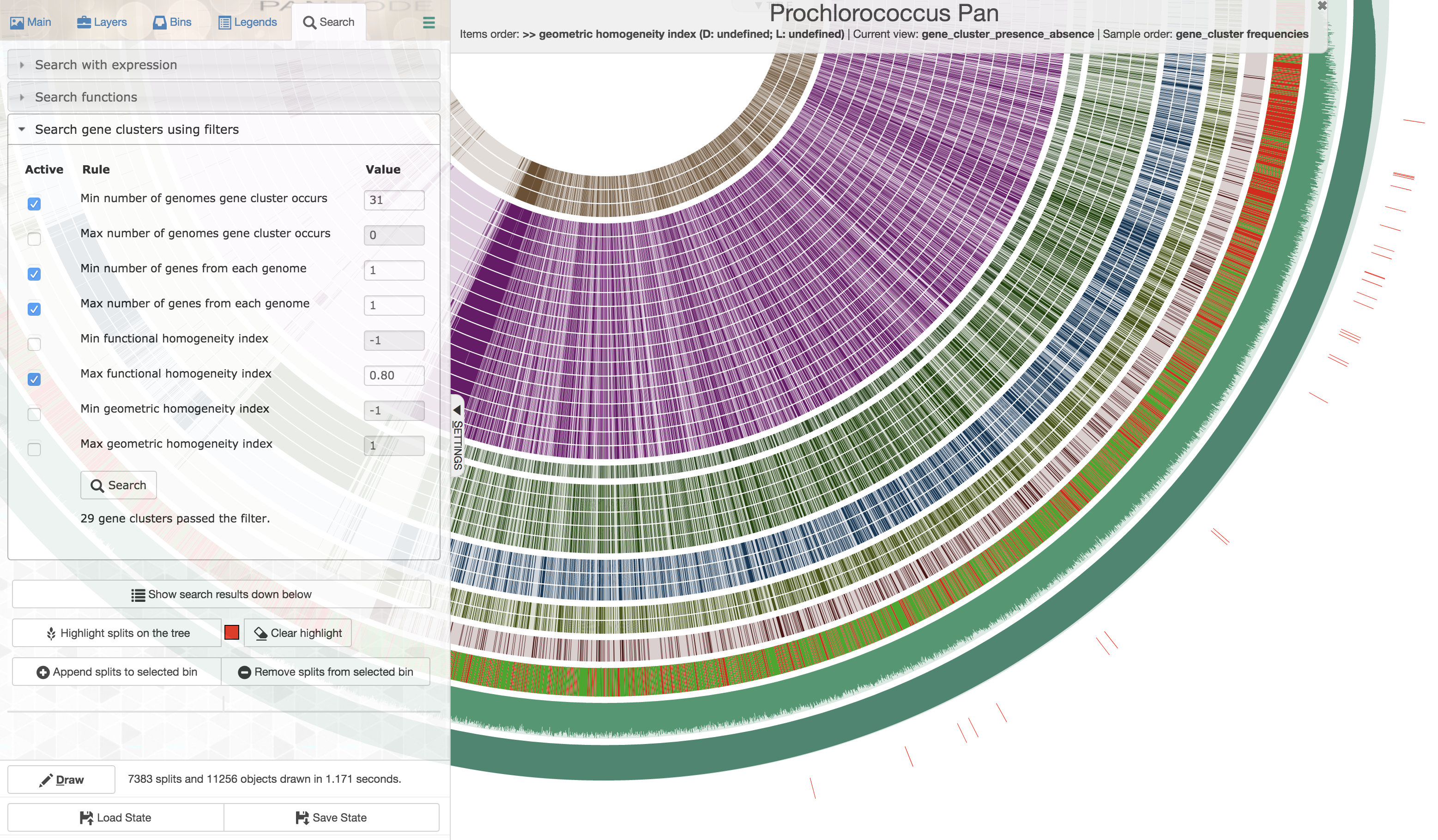
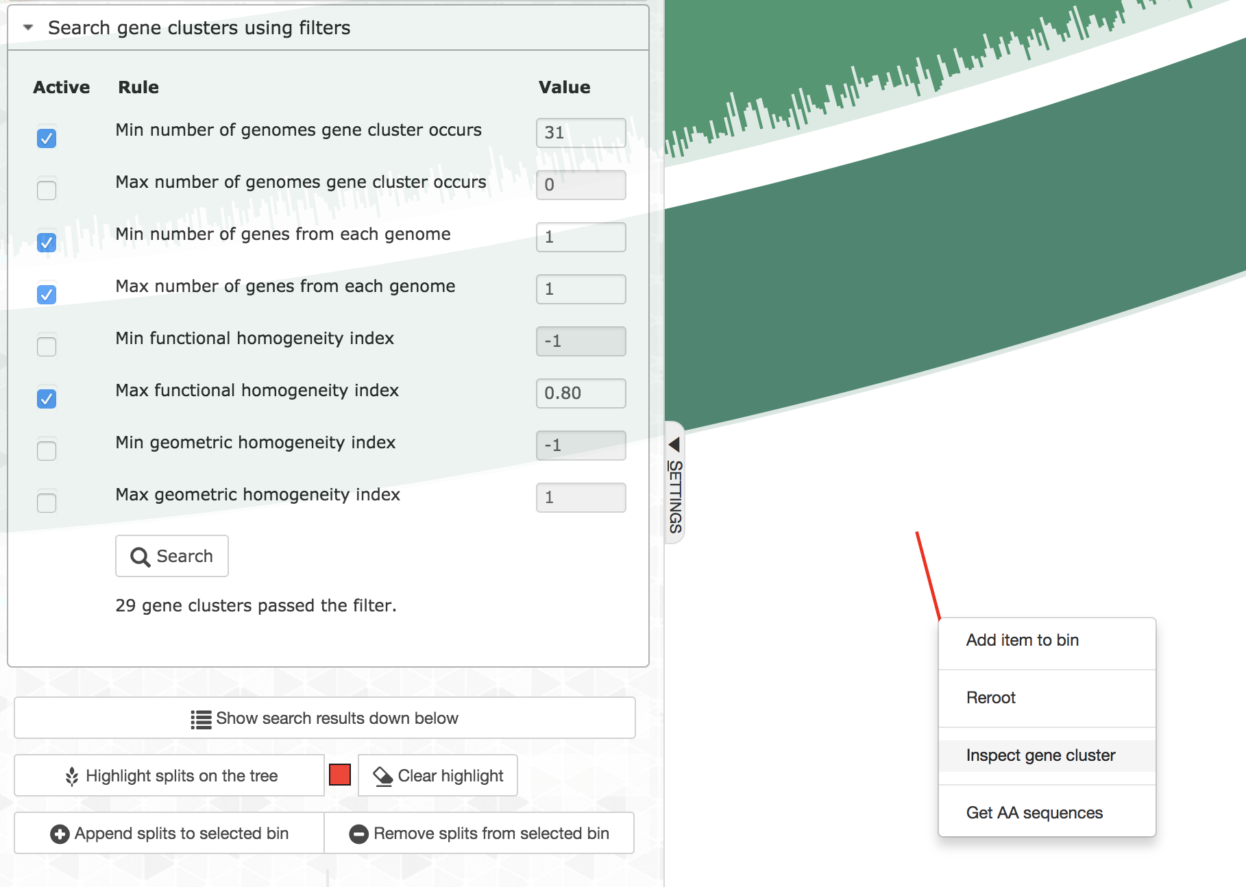
Well, for this very specific set of constraints you could first order all gene clusters based on decreasing geometric homogeneity index, then enter the following values to set up a filter before applying it and highlighting the matching gene clusters:
The first gene cluster in counter-clockwise order is the one that best matches to the listed criteria. Upon closer inspection,
One could see that there is tremendous amount of functional variability among aligned residues across genomes, despite the geometric homogeneity of the sequences in the gene cluster (only a portion of the alignment is shown here):
Those of you who read our study on the topic, would perhaps not be surprised to learn that the COG functional annotation of this particular gene cluster resolves to an enzyme that is related to cell wall/membrane/envelop biogenesis. It is always good when things check out.
Scrutinizing phylogenomics
Here is another example usage of homogeneity indices. We often use single-copy core gene clusters for phylogenomic analyses to estimate evolutionary relationships between our genomes. Identifying single-copy core gene clusters is easy either through advanced filters, or through manual binning of gene clusters:
But single-copy core gene clusters will contain many poorly aligned gene clusters that you may not want to use for a phylogenomic analysis so as to minimize the influence of noise that stems from bioinformatics decisions regarding where to place gaps. On the other hand, there will be many gene clusters that are near-identical in this collection, which would be rather useless to infer phylogenomic relationships. Luckily, you could use homogeneity indices and advanced search options to identify those that are geometrically perfect, but functionally diverse:
You could easily append those that match to these criteria to a separate bin:
And perform a quick-and dirty analysis on-the-fly to see how they would organize your genomes directly on the interface:
Or you could get the FASTA file with aligned and concatenated amino acid sequences for these gene clusters to do a more appropriate phylogenomic analysis:
anvi-get-sequences-for-gene-clusters -p PROCHLORO/Prochlorococcus_Pan-PAN.db \
                                     -g PROCHLORO-GENOMES.db \
                                     -C default -b Better_core \
                                     --concatenate-gene-clusters \
                                     -o better_core.fa
Needless to say, estimates for homogeneity indices per gene cluster will also appear in your summary files from anvi-summarize to satisfy the statistician within you.
Calculating rarefaction curves and Heaps’ Law parameters
Please note that if you are reading these lines when the latest stable version of anvi’o is v8, it means this feature is still only available in anvio-dev branch. Apologies for the inconvenience.
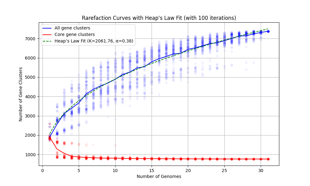
You can use the program anvi-compute-rarefaction-curves to calculate and report rarefaction curves and Heaps’ Law fit for your pangenome.
As described in the program help page, rarefaction curves are helpful in the analysis of pangenome as they help visualize the discovery rate of new gene clusters as a function of increasing number of genomes. While a steep curve suggests that many new gene clusters are still being discovered, indicating incomplete coverage of the potential gene cluster space, a curve that reaches a plateau suggests sufficient sampling of gene cluster diversity.
However, rarefaction curves have inherent limitations. Because genome sampling is often biased and unlikely to fully capture the true genetic diversity of any taxon, rarefaction analysis provides only dataset-specific insights. Despite these limitations, rarefaction curves remain a popular tool for characterizing whether a pangenome is relatively ‘open’ (with continuous gene discovery) or ‘closed’ (where new genome additions contribute few or no new gene clusters). As long as you take such numerical summaries with a huge grain of salt, it is all fine.
Fitting Heaps’ Law to the rarefaction curve provides a quantitative measure of pangenome openness. The alpha value derived from Heaps’ Law (sometimes referred to as gamma in the literature) reflects how the number of new gene clusters scales with increasing genome sampling. There is no science to define an absolute threshold for an open or a closed pangenome. However, pangenomes with alpha values below 0.3 tend to be relatively closed, and those above 0.3 tend to be relatively open. Higher alpha values will indicate increasingly open pangenomes and lower values will identify progressively closed ones.
Running anvi-compute-rarefaction-curves on our Prochlorococcus pangenome the following way,
anvi-compute-rarefaction-curves -p PROCHLORO/Prochlorococcus_Pan-PAN.db \
                                --iterations 100 \
                                -o rarefaction.svg
will result in the following output,
Number of genomes found ......................: 31
Number of iterations to run ..................: 100
Output file ..................................: rarefaction.svg
Heap's Law parameters estimated ..............: K=2061.7563, alpha=0.3762
from which we will learn that our pangenome is relatively ‘open’, and obtain this figure to include in our reporting of this pangenome:
Always generate SVG or PDF outputs to be able to later edit in program such as Inkscape and fit these results into your final figures nicely.
Splitting the pangenome
In some cases one might want to split a given pangenome into multiple independent pangenomes, such as one that contains only core gene clusters, or one that contains only singletons, etc. This advanced functionality is most useful when one wishes to do very high-resolution phylogenomic analyses by scrutinizing core genes in the pangenome with an orchestrated use of functional and geometric homogeneity indices (which can also be done without splitting the pangenome, but we find that it sometimes it makes things easier).
For this we have anvi-split, a multi-talented program to split things, which also works with collections and bins in pan databases. Using this program you can focus on any group of gene clusters that are defined in a bin in a given pangenome, and split them into an independent and stand-alone pangenome.
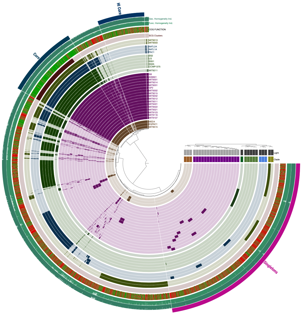
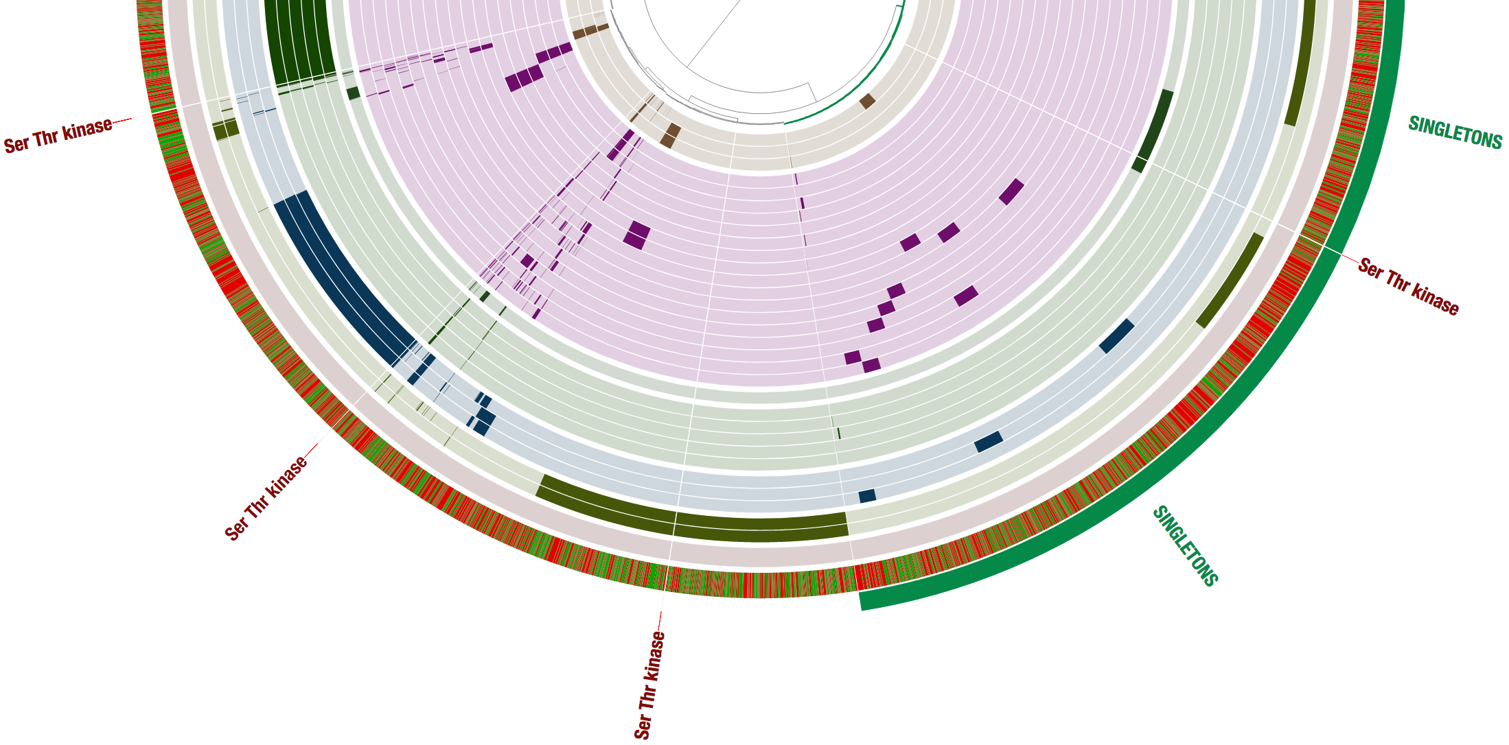
If you are feeling lost, you will likely find the visual description of this functionality much more clear than the technical one. Following steps will demonstrate it using the Prochlorococcus pangenome. Let’s assume in the Prochlorococcus pangenome you happened to have three bins, Core, HL Core, and Singletons, all stored in the collection named default:
These bins can be split from this pangenome into their own little pan databases using anvi-split this way:
anvi-split -p Prochlorococcus-PAN.db \
           -g Prochlorococcus-GENOMES.db \
           -C default \
           -o SPLIT_PANs
The resulting directory would contain the following files:
$ ls -lR SPLIT_PANs
total 0
drwxr-xr-x  3 meren  staff  96 Apr 26 16:37 Core
drwxr-xr-x  3 meren  staff  96 Apr 26 16:37 Hl_Core
drwxr-xr-x  3 meren  staff  96 Apr 26 16:37 Singletons

SPLIT_PANs/Core:
total 3240
-rw-r--r--  1 meren  staff  1658880 Apr 26 16:37 PAN.db

SPLIT_PANs/Hl_Core:
total 1560
-rw-r--r--  1 meren  staff  798720 Apr 26 16:37 PAN.db

SPLIT_PANs/Singletons:
total 4672
-rw-r--r--  1 meren  staff  1384448 Apr 26 16:37 PAN.db
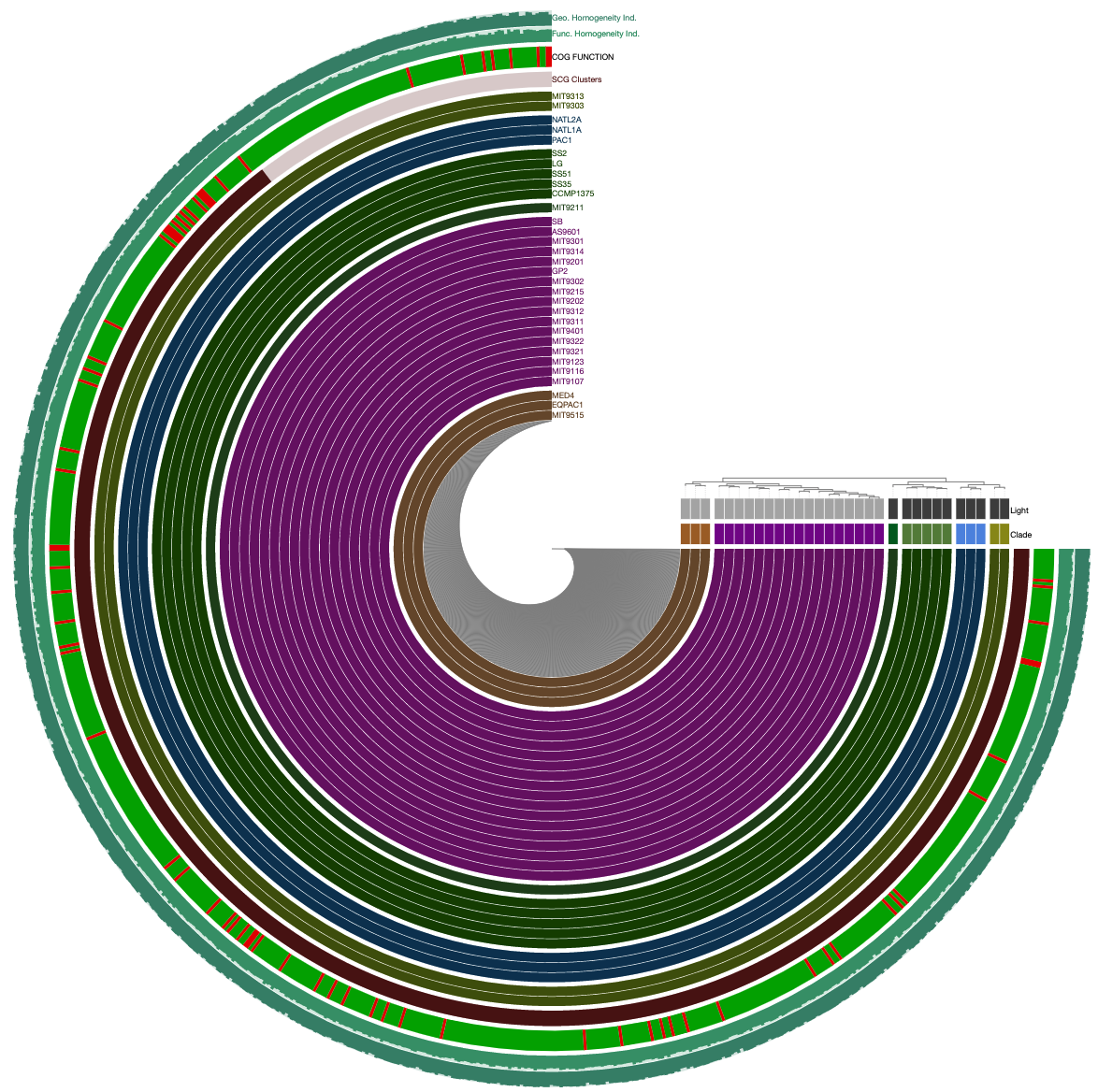
As you can see these are individual pangenomes that can indeed be visualized with anvi-display-pan. For instance running the following command,
anvi-display-pan -p SPLIT_PANs/Core/PAN.db \
                 -g Prochlorococcus-GENOMES.db
Would give you this display:
Or runnig this one instead,
anvi-display-pan -p SPLIT_PANs/Singletons/PAN.db \
                 -g Prochlorococcus-GENOMES.db
Would give you this one:
And that’s that.
Quantifying functional enrichment in a pangenome
Once we have our pangenome, one of the critical things that we usually want to do is look at the functions associated with our gene clusters, especially those that are accessory to subsets of genomes in our pangenome. Anvi’o can help you identify functions that are enriched for some of the clades or sub clades that are included in your pangenome via the program This is done with our new and improved program anvi-compute-functional-enrichment-in-pan.
This program utilizes information you provide by splitting your genoems into multiple grups, and finds functions that are characteristic to any of those groups, i.e. functions that are enriched in genomes that belong to one group, but predominantly absent in genomes outside of it.
To use this feature you must have at least one categorical additional layer information (which can easily be done via anvi-import-misc-data), and at least one functional annotation source for your genomes storage (which will automatically be the case if every contigs database that were used when you run anvi-gen-genomes-storage was annotated with the same functional source). If you are unsure whether there are any functions available to you in your genomes storage, you can run anvi-db-info on it and thake a look at the output.
Alon’s short ‘behind the scenes’ lecture on anvi’o functional enrichment analysis for the curious
For those of you who like to dive into the details, here is some information about what goes on behind the scenes.
In order for this analysis to be compatible with everything else relating to the pangenome, we decided that it should be focused on gene clusters, since they are the heart of our pangenomes. This means that the first step of the functional analysis is to try to associate every gene cluster with a function. This is necessary because gene clusters do not have functional annotation by default, as functional annotation is done in anvi’o at the level of individual genes.
In an ideal world, all genes in a single gene cluster would be annotated with the same identical function. While in reality this is usually the case, it is not always true. In cases in which there are multiple functions associated with a gene cluster, we chose the most frequent function, i.e. the one that the largest number of genes in the gene cluster matches (if there is a tie of multiple functions, then we simply choose one arbitrarily). If none of the genes in the gene cluster were annotated, then the gene cluster has no function associated to it.
Naturally, when we associate each gene cluster with a single function, we could end up with multiple gene clusters in a pangenome with the same function. From our experience, most functions are associated with a single gene cluster, but there are still plenty of functions that associate with multiple gene clusters, and this will be more common in pangenomes that contain distantly related genomes. In these cases, in order to find the occurrence of a given function among genomes, we simply ‘merge’ the occurrences of all gene clusters associated with that same function (for you computational readers, we simply take the sum of the occurrence frequency vectors of the gene clusters across genomes).
The careful readers will notice that we distinguish between ‘functional annotation’ and ‘functional association’ in the following text. When we mention ‘functional annotation’, we refer to the annotation of a single gene with a function by the functional annotation source (i.e. COGs, EggNOG, etc.), whereas ‘functional association’ of a gene cluster is the association of gene clusters with a single function as described above.
Ok, so now we have a frequency table of functions in genomes and we use it as an input to the functional enrichment test. This test was implemented by Amy Willis in R (you can find the script here), and uses a Generalized Linear Model with the logit linkage function to compute an enrichment score and p-value for each function. False Detection Rate correction to p-values to account for multiple tests is done using the package qvalue.
In addition to the enrichment test, we use a simple heuristic to find the groups that associate with each function. This association is only meaningful for functions that are truly enriched, and should otherwise be ignored. We simply determine that for every function, the associated groups are the ones in which the occurrence of the function of genomes is greater than the expected occurrence under a uniformal distribution (i.e. if the function was equally probable to occur in genomes from all groups). Mathematically speaking (if you are into that kind of stuff), if we denote \(E_{ij}\) as the expected number of genomes in group \(i\) with the function \(j\) under the null distribution, where we consider the null distribution to be a uniform distribution. Hence:
\[\begin{equation}\label{eq:expected_occurrence} E_{ij} = \frac{n_i}{\sum_{i'=1}^N n_{i'}} \cdot \sum_{i'=1}^N O_{i'j} \end{equation}\]And we denote the actual occurrence of function \(j\) in group \(i\) as \(O_{ij}\), then we consider the associated groups as one where \(O_{ij} > E_{ij}\).
Now we can use all this information to explore our data, see the details below!
Let’s use the Prochlorococcus example to learn what we can do with this.
First we will compare the low-light vs. the high-light genomes in order to see if there are any functions that are unique to either group using the ‘light’ categorical additional layer data (if this doesn’t make sense to you please go back to one of the pangenome figures above and see the layer additional data ‘light’):
anvi-compute-functional-enrichment-in-pan -p PROCHLORO/Prochlorococcus_Pan-PAN.db \
                                          -g PROCHLORO-GENOMES.db \
                                          --category light \
                                          --annotation-source COG14_FUNCTION \
                                          -o enriched-functions.txt
Here is the structure of the output file enriched-functions.txt (there are more columns, scroll towards right to see them):
| COG14_FUNCTION | enrichment_score | unadjusted_p_value | adjusted_q_value | associated_groups | accession | gene_clusters_ids | p_LL | p_HL | N_LL | N_HL |
|---|---|---|---|---|---|---|---|---|---|---|
| 1,6-Anhydro-N-acetylmuramate kinase | 31.00002278725133 | 2.5802540103336397e-8 | 1.702967646820229e-6 | LL | COG2377 | GC_00001726 | 1 | 0 | 11 | 20 |
| GTPase Era, involved in 16S rRNA processing; Uncharacterized conserved protein, DUF697 family | 31.00002278725133 | 2.5802540103336397e-8 | 1.702967646820229e-6 | LL | COG1159; COG3597 | GC_00001780 | 1 | 0 | 11 | 20 |
| N-acetylglucosamine-6-phosphate deacetylase | 31.00002278725133 | 2.5802540103336397e-8 | 1.702967646820229e-6 | LL | COG1820 | GC_00001771 | 1 | 0 | 11 | 20 |
| Exonuclease VII small subunit | 31.00002278725133 | 2.5802540103336397e-8 | 1.702967646820229e-6 | LL | COG1722 | GC_00002650, GC_00003618, GC_00004698, GC_00006635 | 1 | 0 | 11 | 20 |
| Periplasmic beta-glucosidase and related glycosidases | 31.00002278725133 | 2.5802540103336397e-8 | 1.702967646820229e-6 | LL | COG1472 | GC_00002098, GC_00003920 | 1 | 0 | 11 | 20 |
| 3-hydroxyisobutyrate dehydrogenase or related beta-hydroxyacid dehydrogenase | 31.00002278725133 | 2.5802540103336397e-8 | 1.702967646820229e-6 | LL | COG2084 | GC_00002015, GC_00003562 | 1 | 0 | 11 | 20 |
| Exonuclease VII, large subunit | 31.00002278725133 | 2.5802540103336397e-8 | 1.702967646820229e-6 | LL | COG1570 | GC_00001723 | 1 | 0 | 11 | 20 |
| Na+/proline symporter | 31.00002278725133 | 2.5802540103336397e-8 | 1.702967646820229e-6 | LL | COG0591 | GC_00001786 | 1 | 0 | 11 | 20 |
| Uncharacterized integral membrane protein | 31.00002278725133 | 2.5802540103336397e-8 | 1.702967646820229e-6 | LL | COG5413 | GC_00002085, GC_00002286, GC_00003831 | 1 | 0 | 11 | 20 |
| (…) | (…) | (…) | (…) | (…) | (…) | (…) | (…) | (…) | (…) | (…) |
The following describes each column in this output:
-
COG14_FUNCTION this column has the name of the specific function for which enrichment was calculated. In this example we chose to use
COG14_FUNCTIONfor functional annotation, and hence the column title isCOG14_FUNCTION. You can specify whichever functional annotation source you have in your PAN database using the--annotation-source, and then the analysis would be done according to that annotation source. Even if you have multiple functional annotation sources in your genome storage, only one source could be used for a single run of this program. If you wish, you could run it multiple times and each time use a different annotation source. If you don’t remember which annotation sources are available in your genomes storage, you can use the flag--list-annotation-sources. -
enrichment_score is a score to measure how much is this function unique to the genomes that belong to a specific group vs. all other genomes in your pangenome. This score was developed by Amy Willis. For more details about how we generate this score, see the note from Amy below.
-
unadjusted_p_value is the p-value for the enrichment test (unadjusted for multiple tests).
-
adjusted_q_value is the adjusted q-value to control for False Detection Rate (FDR) due to multiple tests (this is necessary since we are running the enrichment test each function separately).
-
associated_groups is the list of groups (or labels) in your categorical data that are associated with the function. Notice that if the enrichment score is low, then this is meaningless (if the function is not enriched, then it is not really associated with any specific group/s). See Alon’s explanation above to understand how these are computed.
-
function_accession is the function accession number.
-
gene_clusters_ids are the gene clusters that were associated with this function. Notice that each gene cluster would be associated with a single function, but a function could be associated with multiple gene clusters.
-
p_LL, p_HL for each group (in the case of this example there are two groups:
LLandLH) there will be a column with the portion of the group members in which we detected the funtion. -
N_LL, N_HL for each group these columns specify the total number of genomes in the group.
Our example here includes only two categories (LL and HL), but you can have as many different categories as you want. Just remember that if some of your groups have very few genomes in them, then the statistical test will not be very reliable. The minimal number of genomes in a group for the test to be reliable depends on a number of factors, but we recommend proceeding with great caution if any of your groups have fewer than 8 genomes.
A note from Amy Willis regarding the functional enrichment score
The functional enrichment score proposed here and implemented in anvi’o is the Rao test statistic for equality of proportions. Essentially, it treats each category (here, high light and low light) as an explanatory variable in a logistic regression (binomial GLM), and tests the significance of the categorical variable in explaining the occurrence of the function.
The test accounts for the fact that there may be more genomes observed from one category than the other. As usual, having more genomes makes the test more reliable. There are lots of different ways to do this test, but we did some investigations and found that the Rao test had the highest power out of all tests that control Type 1 error rate. Yay!
Since many users will be looking at testing for enrichment across many functions, by default we adjust for multiple testing by controlling the false discovery rate. For this reason, please report q-values instead of p-values in your paper if you use this statistic.
Now let’s search for one of the top functions in the table “Ser/Thr protein kinase RdoA involved in Cpx stress response, MazF antagonist”, which is enriched for the members of the LL group, and we can see in the table that it matches four gene clusters.
In fact, if we look carefully, then we find that this function matches a gene cluster that is unique for each one of the four low light clades, and is a single-copy core gene for the low light genomes in our pangenome. Cool!
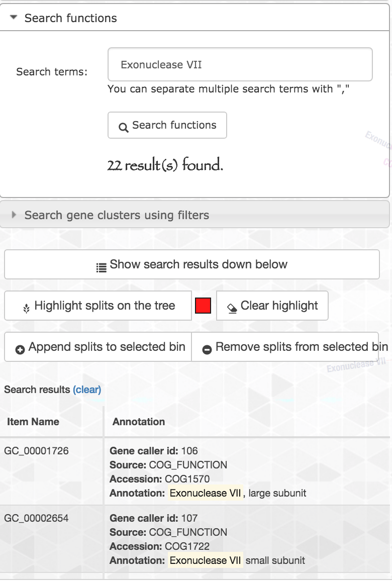
Let’s look at another enriched function: Exonuclease VII, large subunit. When we search this function, we should be careful since the name of the function contains a comma, and the function search option in the interactive interface treats the comma as if it is separating multiple functions that are to be searched at the same time. Hence I just searched for Exonuclease VII, and here are the results:
We can see that the search matched hits for both Exonuclease VII, large and small subunits, with a total of 22 hits.
The large subunit matches a single gene cluster which is in the CORE LL, and the small subunit matches a gene cluster in each one of the clade specific cores (similar to what we saw above for the Ser/Thr protein kinase). Both of these genes are also part of the single copy core unique to low light members and absent from high light members.
Computing the average nucleotide identity for genomes (and other genome similarity metrics too!)
Anvi’o also contains a program, anvi-compute-genome-similarity, which uses various similarity metrics such as PyANI to compute average nucleotide identity across your genomes, and sourmash to compute mash distance across your genomes. It expects any combination of external genome files, internal genome files, or a fasta text file that points to the paths of FASTA files (each FASTA is assumed to be 1 genome). In addition, anvi-compute-genome-similarity optionally accepts a pan-db to add all results into it as additional layer data.
Here is an example with our Prochlorococcus pangenome:
anvi-compute-genome-similarity --external-genomes external-genomes.txt \
                               --program pyANI \
                               --output-dir ANI \
                               --num-threads 6 \
                               --pan-db PROCHLORO/Prochlorococcus_Pan-PAN.db
Once it is complete, we can visualize the pan genome using anvi-display-pan again to see what is new:
anvi-display-pan -g PROCHLORO-GENOMES.db \
                 -p PROCHLORO/Prochlorococcus_Pan-PAN.db
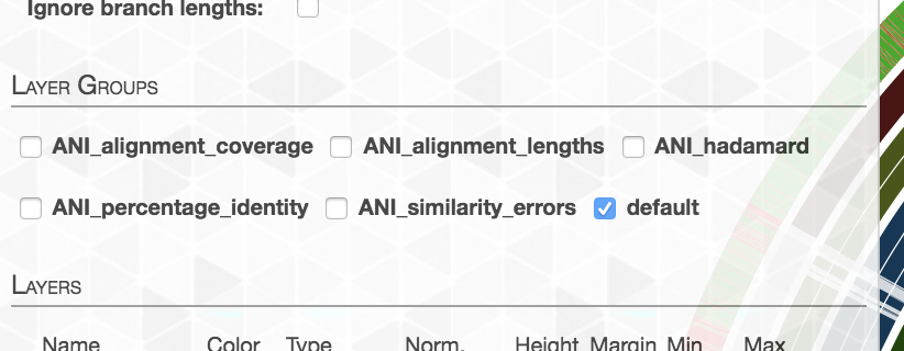
When you first look at it you will not see anything out of ordinary. But if you go to the ‘Layers’ tab, you will see the following addition:
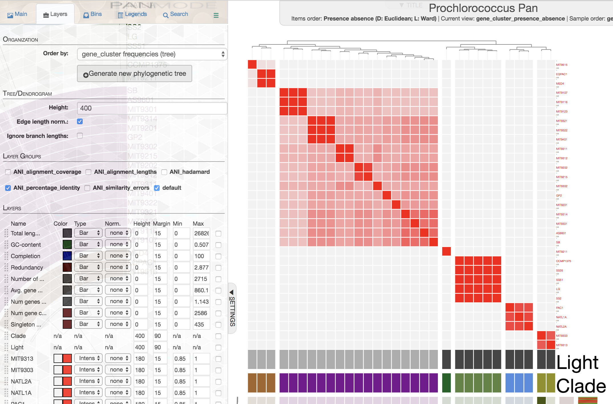
If you click the checkbox for, say, ANI_percentage_identity, you will see a new set of entries will be added into the list of layer data entries. Then, if you click the button ‘Draw’ or ‘Redraw layer data’, you should see the ANI added to your display:
Yes. Magic.
You may need to change the min value from the interface for a better representation of ANI across your genomes in your own pangenome.
A little note from Meren on how to order genomes
It has always been a question mark for me how to order genomes with respect to gene clusters. Should one use the gene cluster presence/absence patterns to organize genomes (where one ignores paralogs and works with a binary table to cluster genomes)? Or should one rely on gene cluster frequency data to order things (where one does consider paralogs, so their table is not binary anymore, but contains the frequencies for number of genes from each genome in each gene cluster)?
Thanks to Özcan’s new addition to the codebase, I’ve made an unexpected observation while I was working on this section of the tutorial regarding this question of ‘how to order genomes’ in a pangenome.
This is how ANI matrix looks like when I order Prochlorococcus genomes based on gene cluster frequency data:
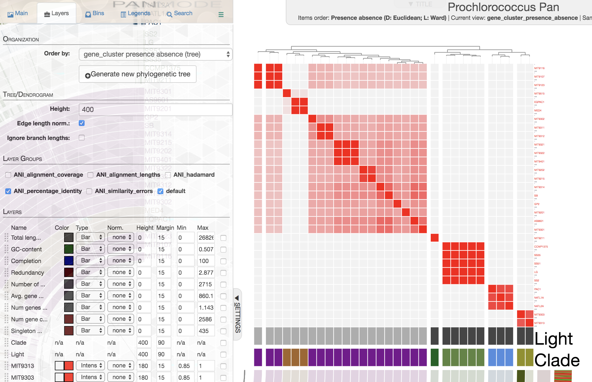
In contrast, this is how ANI matrix looks like when I order genomes based on gene cluster presence/absence data:
There you have it.
If you are working with isolate genomes, maybe you should consider ordering them based on gene cluster frequencies since you would expect a proper organization of genomes based on gene clusters should often match with their overall similarity. Here are some small notes:
-
In this case it is easy to see that organization by gene cluster presence/absence data is doing a poor jobby mixing up high-light group II (purple) and high-light group I (poopcolor) genomes. We can identify the problem clealry because we know the clades to which these genomes belong, in cases where you have no idea about these relationships, it seems gene cluster frequencies can organize your genomes more accurately.
-
It is sad to know that MAGs will often lack multi-copy genes, and they will have less paralogs (since assembly of short reads create very complex de Bruijn graphs which obliterate all redundancy in a given genome), hence their proper organization will not truly benefit from gene cluster frequency data, at least not as much as isolate genomes, and the errors we see with gene cluster presence/absence data-based organization will have a larger impact on our pangenomes.
-
See the emergence of those sub-clades in high-light group II? If you are interested, please take a look at our paper on Prochlorococcus metapangenome (especially the section “The metapangenome reveals closely related isolates with different levels of fitness”), in which we divided HL-II into multiple subclades and showed that despite small differences between these genomes, those sub-clades displayed remarkably different environmental distribution patterns. The sub-clades that we could define in that study based on gene cluster frequencies and environmental distribution patterns match quite well to the groups ANI reveals. This goes back to some of the most fundamental questions in microbiology regarding how to define ecologically relevant units of microbial life. I don’t know if we are any close to making any definition, but I can tell you that those ‘phylogenetic markers’ we are using … I am not sure if they are really working that well (smiley).
Summarizing an anvi’o pan genome
When you store your selections of gene clusters as a collection, anvi’o will allow you to summarize these results.
Even if you want to simply summarize everything in the pan genome without making any selections in the interface, you will still need a collection in the pan database. But luckily, you can use the program anvi-script-add-default-collection to add a default collection that contains every gene cluster.
The summary step gives you two important things: a static HTML web page you can compress and share with your colleagues or add into your publication as a supplementary data file, and a comprehensive TAB-delimited file in the output directory that describes every gene cluster.
You can summarize a collection using the program anvi-summarize, and a generic form of this command looks like this:
$ anvi-summarize -p PROJECT-PAN.db \
                 -g PROJECT-PAN-GENOMES.db \
                 -C COLLECTION_NAME \
                 -o PROJECT-SUMMARY
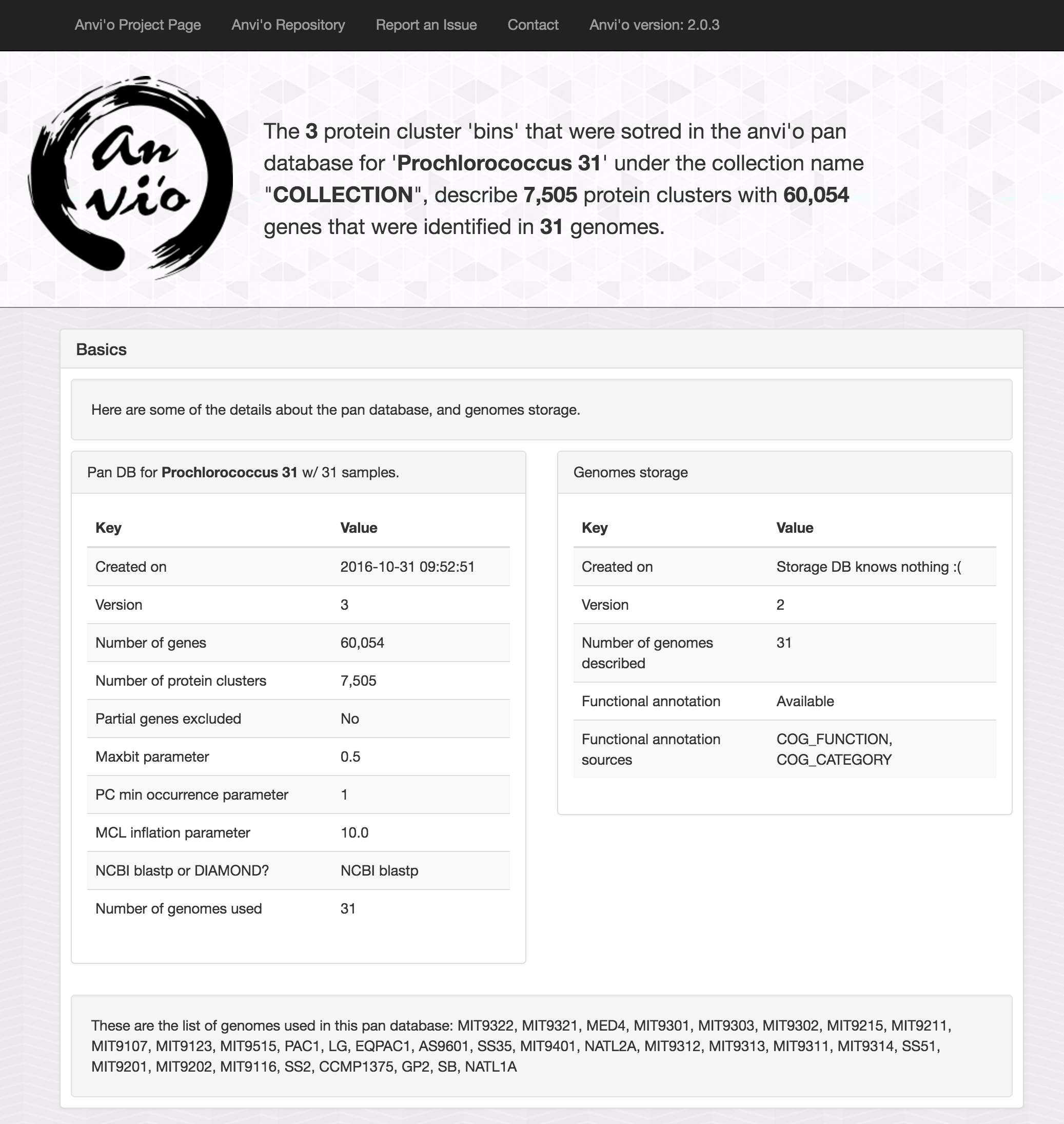
If you open the index.html file in the summary directory, you will see an output with some essential information about the analysis:
As well as the TAB-delimited file for gene clusters:
The structure of this file will look like this, and will give you an opportunity to investigate your gene clusters in a more detailed manner (you may need to scroll towards right to see more of the table):
| unique_id | gene_cluster_id | bin_name | genome_name | gene_callers_id | COG_FUNCTION_ACC | COG_FUNCTION | COG_CATEGORY_ACC | COG_CATEGORY | aa_sequence |
|---|---|---|---|---|---|---|---|---|---|
| 1 | PC_00001990 | MIT9303 | 30298 | COG1199 | Rad3-related DNA helicase | L | Replication, recombination and repair | MLEARSHQQLKHLLLQNSSP(…) | |
| (…) | (…) | (…) | (…) | (…) | (…) | (…) | (…) | (…) | (…) |
| 91 | PC_00001434 | Core_HL | MIT9322 | 42504 | COG3769 | Predicted mannosyl-3-phosphoglycerate phosphatase | G | Carbohydrate transport and metabolism | MIENSSIWVVSDVDGTLMDH(…) |
| (…) | (…) | (…) | (…) | (…) | (…) | (…) | (…) | (…) | (…) |
| 257 | PC_00000645 | Core_all | MIT9322 | 42217 | COG1185 | Polyribonucleotide nucleotidyltransferase | J | Translation, ribosomal structure and biogenesis | MEGQNKSITFDGREIRLTTG(…) |
| (…) | (…) | (…) | (…) | (…) | (…) | (…) | (…) | (…) | (…) |
| 2019 | PC_00001754 | Core_LL | NATL2A | 49129 | COG0127 | Inosine/xanthosine triphosphate pyrophosphatase | F | Nucleotide transport and metabolism | MDNVPLVIASGNKGKIGEFK(…) |
| (…) | (…) | (…) | (…) | (…) | (…) | (…) | (…) | (…) | (…) |
| 5046 | PC_00001653 | PAC1 | 52600 | COG1087 | UDP-glucose 4-epimerase | M | Cell wall/membrane/envelope biogenesis | MRVLLTGGAGFIGSHIALLL(…) | |
| 5047 | PC_00001653 | LG | 7488 | COG1087 | UDP-glucose 4-epimerase | M | Cell wall/membrane/envelope biogenesis | MNRILVTGGAGFIGSHTCIT(…) | |
| 5048 | PC_00001653 | SS35 | 56661 | COG1087 | UDP-glucose 4-epimerase | M | Cell wall/membrane/envelope biogenesis | MNRILVTGGAGFIGSHTCIT(…) | |
| 5049 | PC_00001653 | NATL2A | 49604 | COG1087 | UDP-glucose 4-epimerase | M | Cell wall/membrane/envelope biogenesis | MRVLLTGGSGFIGSHVALLL(…) | |
| (…) | (…) | (…) | (…) | (…) | (…) | (…) | (…) | (…) | (…) |
This file will link each gene from each genome with every selection you’ve made and named through the interface or through the program anvi-import-collection, and will also give you access to the amino acid sequence and function of each gene.
Creating a pangenome with functions
It is also possible to define gene clusters based on gene functions rather than gene sequences. This may be a useful way to compare genomes that are too distant for high-resolution analyses with pangenomics. For such applications, please see the program anvi-display-functions


