


Table of Contents
Introduction
My goal in this document is to demonstrate the components of the oligotyping pipeline, so you feel familiar with it. If you would like to learn about how to oligotype, Best Practices would be a better article to read.
I came up with a mock problem to solve by using the pipeline, but I would strongly suggest you to read some of the studies that used oligotyping to get a better sense. A short but comprehensive list can be found here.
Mock example
Going back to the mock example, here is the problem: Lets assume we have 10 samples collected from 10 different environments. Lets say the first 5 samples were collected during the summer, and the last 5 were collected during the winter. Assume the taxonomy analysis shows that Pelagibacter (SAR 11) is present in all samples. And these are the questions we wish to answer:
- “Are all Pelagibacter in all 10 samples the same?”,
- and “if there are different types, how are they distributed?”.
In order to make a good case, I generated 10 samples, each containing 250 sequences, using 2 strains from Pelagibacter that differ from each other by 2 nucleotides (considering the sequence length, these two strains are 99% identical at the 16S rRNA gene region we sequenced). By using these two strains as a template, I generated the FASTA file below by using pommunity (pommunity is a simple tool I implemented to generate pseudo communities with expected sequencing errors based on the literature on 454 (Roche Genome Sequencer FLX)):
http://oligotyping.org/sample-run/mock-env.fasta
By using pommunity, I introduced random sequencing errors, so they look just like what we would expect to see if we had isolated these reads from an actual 454 run.
These 10 samples contain two different types of Pelagibacter. Also, the ratio of two types of Pelagibacter in these samples are different: the first 5 samples are composed of 91% of type 1 strain and 9% of type 2 strain, while the last 5 samples are composed of 9% percent type 1 strain and 91% type 2 strain.
At this point you know everything about the content of this FASTA file. If you are up for a challenge, you can play with this FASTA file by using your favorite tools to extract the information I just explained. I already tried a couple of things: if you use RDP or GAST, you will have all these reads assigned to Pelagibacter. If you would use UCLUST to cluster them, you will get 4 clusters at 97%, and 169 clusters at 99% identity level.
Getting the Pipeline Going
Installation
For installation instructions, please refer to this post:
https:merenlab.org/2014/08/16/installing-the-oligotyping-pipeline/
Alternatively you may acquire the virtual machine and get the pipeline running without an installation:
https:merenlab.org/2014/09/02/virtualbox/
Preparing the FASTA file
The oligotyping pipeline requires the input FASTA file to be formatted in a certain way.
It is not complicated, but it is a requirement for running the pipeline properly. First, all of your reads from all of your samples of interest have to be in a single FASTA file, and all reads have to have deflines formatted in the following format:
 >Sample-01_ReadX
 GTTGAAAAAGTTAGTGGTGAAATCCCAGA
 >Sample-01_ReadY
 GTTGAAAAAGTTAGTGGTGAAATCCCAGA
 >Sample-01_ReadZ
 GGTGAAAAAGTTAGTGGTGAAATCCCAGA
 >Sample-02_ReadN
 GTTGAAAAAGTTAGTGGTGAAATCCCAGA
 >Sample-02_ReadM
 GTTGAAAAAGTTAGTGGTGAAATCCCAGA
Are you not sure whether your FASTA file is formatted properly?. Run o-get-sample-info-from-fasta on it. If you see your sample names and expected number of reads in them, you are golden!
The Alignment
Note: Please, please read this article to better undersatnd what alignment means for the oligotyping.
Because we are working with amplicon sequences, our reads are already aligned in a sense (since, thanks to our primers, they are all coming from an evolutionarily homologous region of all genomes we found in our samples). I will try to give a practical recap here, but please read the “Materials and methods” section of the oligotyping methods paper for a much better description of why and when alignment is necessary.
There is one rule: all your reads should have the same length.
It is very easy if you are working with fixed length Illumina reads (such as 100nt long V4 reads on HiSeq), they are already aligned: you can just discard reads that were trimmed during the QC and work with Illumina reads without aligning them. If you are working with Illumina reads merged at the partial overlap (such as V4-V5 on MiSeq), you can just use o-pad-with-gaps script to simply add gaps to short reads in your file to match their length to the longest read in the file. This is perfectly enough, because Illumina does not suffer from insertion/deletion errors, and any length variation is biologically relevant if no QC trimming was performed.
On the other hand, if you are working with Roche/454 reads, your reads will most likely have variable lengths not only due to natural variation among different taxa, but also due to the vast amount of in/del errors 454 introduced. Oligotyping pipeline is not accustomed to deal with this type of length variation, and artificial in/del errors can’t be fixed by simply trimming all reads to the same length. Because trimming 454 reads without alignment will not ameliorate shifts in 454 reads due to homo-polymer region-associated in/del problems. This is when the alignment is necessary. But don’t despair.
Since our mock example is generated with Roche/454 reads, I will continue with the alignment to show you how it could be done easily.
Alignment is an important step and needs to be done carefully. Alignment results will impact the analysis results downstream, however these impacts will mostly remain within alpha diversity estimates. There are many different ways to align a collection of sequences. But I suggest aligning reads against a template for the purpose of preparing them for oligotyping. PyNAST does a great job with GreenGenes alignment templates, and that is what I suggest. Here is the GreenGenes alignment file that you can download and use: gg_97_otus_6oct2010_aligned.fasta.
Once you align all your reads, you can trim them to the same length.
Note: If you use PyNAST and GreenGenes alignments, your resulting aligned sequences will contain many uninformative gaps. You may want to clear those gaps before the entropy analysis. You can use o-trim-uninformative-columns-from-alignment script.
For our mock problem I explained in the Introduction section, I am going to use Muscle to align sequences in the FASTA file. But please stick with PyNAST and don’t use multiple sequence aligners. This is how I run Muscle:
meren ~/tmp/sample-run $ muscle -in mock-env.fasta -out mock-env-aligned.fasta -diags -maxiters 4
In the next section I am going to be using the result of Muscle alignment, mock-env-aligned.fasta, for entropy analysis.
Shannon Entropy Analysis
The first step of oligotyping is to perform Shannon entropy analysis on the aligned sequences. By using Shannon entropy, we are quantifying the uncertainty among the columns of our alignment. Since our goal is to find out the most variable locations in our very closely related taxa to decompose them into meaningful groups, we really want to know how many components there are that are contributing to the uncertainty. Basically, the result of the entropy analysis helps us determine the appropriate number of components to identify oligotypes. Assume I have a directory called ‘sample-run‘ at the same level of oligotyping directory (the directory where the oligotyping codebase resides), and the alignment file that will undergo the entropy analysis (mock-env-aligned.fasta in this example) is in the ‘sample-run‘ directory. Then, this would be the command line to perform entropy analysis on this alignment:
meren ~/tmp/sample-run $ entropy-analysis mock-env-aligned.fasta
Performing entropy analysis: 100%
Once the entropy analysis is finished, you are going to see an entropy distribution figure. For mock-env-aligned.fasta, it should look like this one:
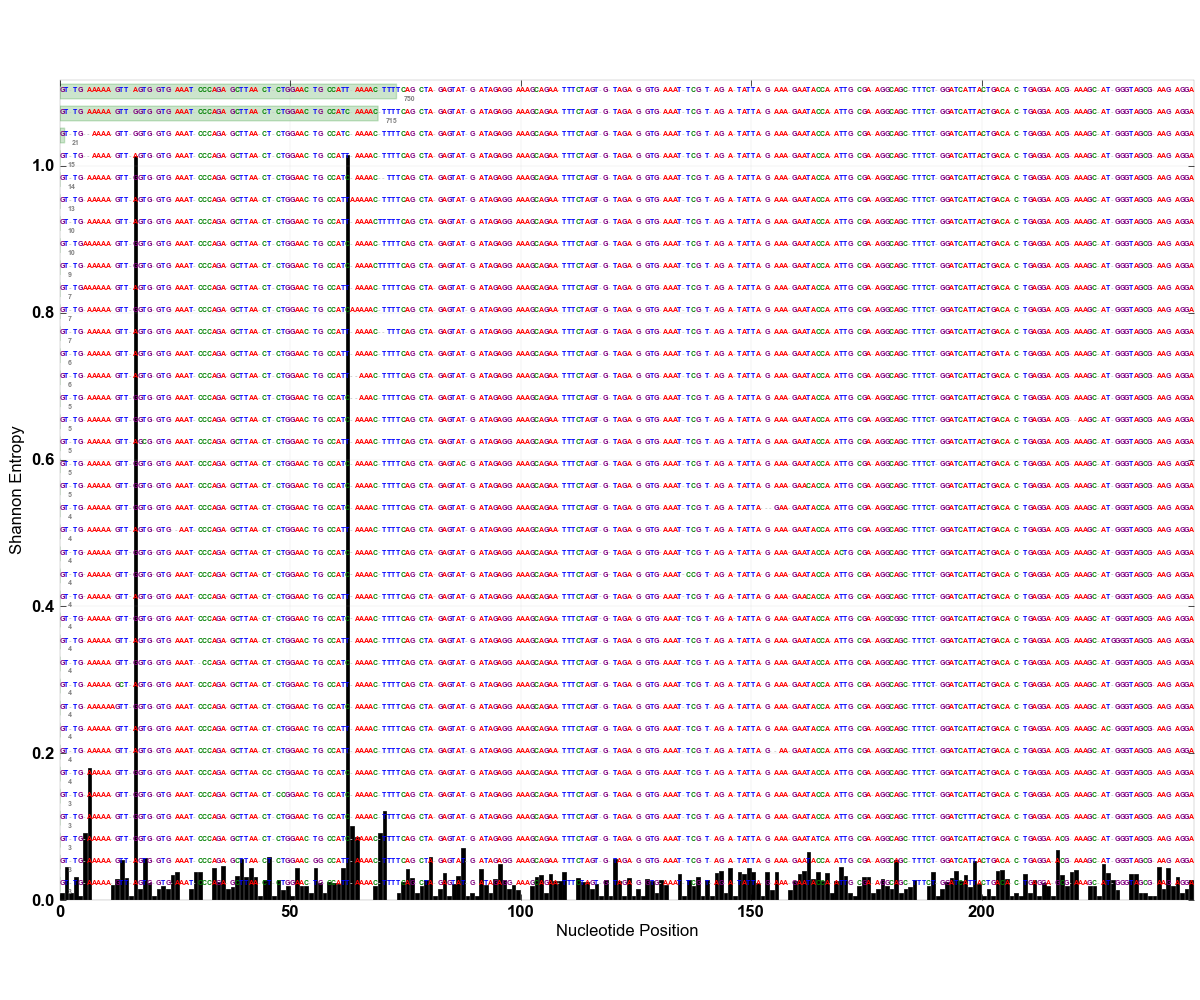
If you recall the explanation of the nature of these sequences from the Introduction section, this figure will make much more sense. We had two types of Pelagibacter that differ from each other by two nucleotides. Entropy analysis shows, along with all the random sequencing errors down below, these two nucleotide positions are the ones that offer the most relevant information to separate these reads from each other. This means, if we use only nucleotides from these two positions, instead of using the entirety of our reads, we can generate distribution profiles for different types.
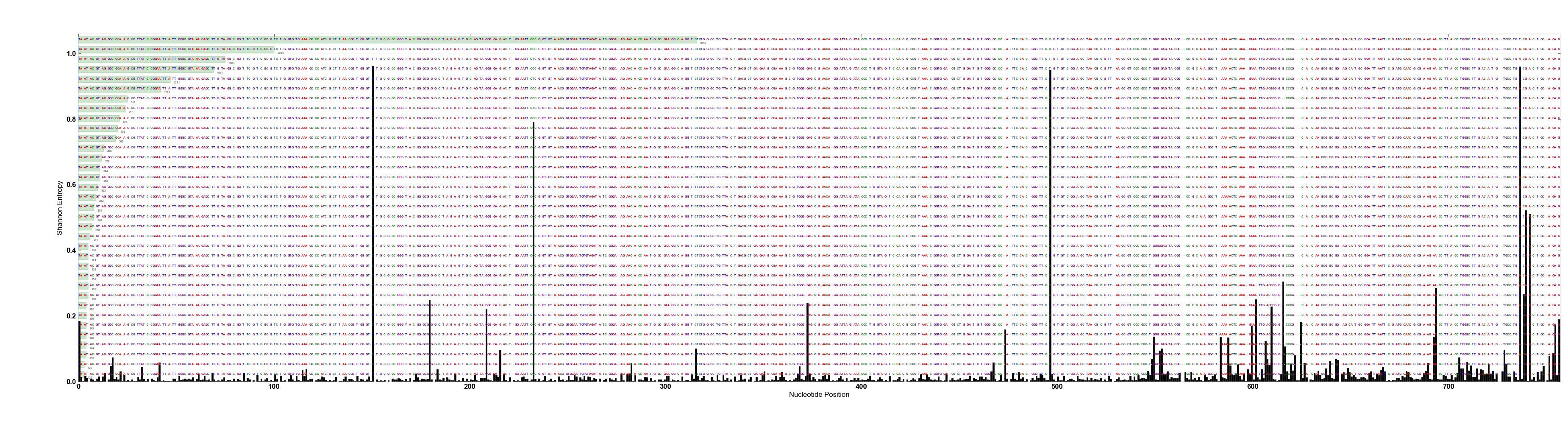
From the figure, it is easy to say that there are two nucleotide positions in this alignment that show high variation. Then, we can assume that using the top two components for oligotyping analysis will be sufficient to decompose those different types from each other. Even though usually it is not this clear cut, real world data present similar stories. Obviously the number of entropy peaks and their volume changes depending on the taxonomic depth you have used to isolate your ‘closely related taxa‘ at the beginning of the analysis. For instance, the following figure shows a real-world case where ~65K pyrotag reads from V3-V5 amplicons that were classified as Gardnerella vaginalis with 99+% identity to a group of known G. vaginalis sequences (click here for more information on G. vaginalis study, which was published recently):
The figure that shows the entropy distribution will be stored as a PNG file in the work directory.
The second product of the entropy analysis step is a text file that contains entropy values for every position in the alignment file. It also will be stored in the work directory:
meren ~/tmp/sample-run $ ls
mock-env-aligned.fasta
mock-env-aligned.fasta-ENTROPY
mock-env-aligned.fasta-ENTROPY.png
This file (mock-env-aligned.fasta-ENTROPY in this case) will be the input of the next step, where the oligotyping pipeline will decompose our closely related taxa and show their distribution among our samples.
Oligotyping
Now the entropy analysis is complete, and we know the number of initial components to use (which is 2, for our Pelagibacter example). At this stage we will be using oligotype program for the analysis, which is a part of the codebase and has many command line options.
You can always see available command line options by typing python oligotype --help.
Oligotyping pipeline can offer a very quick overlook, as well as an extensive analysis that requires more time but provides many essential output files for a deeper analysis.
A Quick Overlook
Oligotyping analysis may take some time depending on the complexity of data, the number of components that are used, and various user requests. However, it is possible to do a very quick analysis and get an idea by sending --quick directive to the pipeline as a parameter. If we go back to our mock-env-aligned.fasta, we already know based on the entropy analysis results, the initial number of components we should be interested is 2. So, if we’d like to oligotype this dataset by using 2 maximum entropy components, this is the command line we need (assuming that you are in the sample-run directory):
oligotype mock-env-aligned.fasta mock-env-aligned.fasta-ENTROPY -c 2 -M 10 --quick
Important note: Before we continue I would like to clarify something: The purpose of this article is to demonstrate the pipeline and help you understand how it works. Your analysis will require different parameters, and you should not copy-paste these commands to analyze your data.
Even more important note: For instance, in no real world analysis you will use -c to generate your final results. Please see Best Practices article to have a better sense of a proper oligotyping analysis and supervision.
First parameter in the command above is the aligned FASTA file, while the second one is the entropy file that was generated during the entropy analysis step. -c indicates the number of components to be used; -M is the minimum subtantive abundance parameter that is used for noise filtering (which I will talk about later). Finally, the --quick directive tells the oligotyping pipeline to produce results as quickly as possible, without generating any figures or output files that are necessary for further supervision.
What files are generated by this run? If you type ls in your work directory, you will realize that there is a new directory created by the oligotyping pipeline called mock-env-aligned-c2-s1-a1.0-A0-M0 (this directory name is actually a combination of the file we analyzed and parameters we used), and here is what you have in that directory:
meren ~/tmp/sample-run $ ls mock-env-aligned-c2-s1-a1.0-A0-M0/
COLORS                MATRIX-COUNT.txt      OLIGOS.nexus          RUNINFO.cPickle
ENVIRONMENT.txt       MATRIX-PERCENT.txt    READ-DISTRIBUTION.txt RUNINFO.log
FIGURES/              OLIGOS.fasta          RUNINFO
Although you will not find anything in the FIGURES directory (due to the use of thanks to the --quick flag), you can visualize your results in the simplest form by typing the following command:
o-stackbar.R mock-env-aligned-c2-s1-a0.0-A0-M10/ENVIRONMENT.txt -o mock --title Mock
As a result of this command a new file, mock.pdf, would be generated in the output directory, which would look like this:
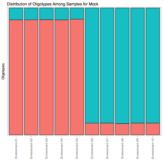
If you remember the nature of the input data from the Introduction section, you should be able to appreciate what you see in this figure:
- Every bar in this stacked bar figure represents a sample in the dataset (from Environment-01 to -10).
- Different colors represent different oligotypes within these samples that are decomposed by using two maximum entropy components.
- The relative abundance of a color in a sample is proportional to the percent abundance of the oligotype that is denoted by that color.
This is an important result, showing that we managed to identify 2 different strains that are 99% identical at the 16S rRNA gene region of interest.
Let’s go back to the contents of the output directory.
One of the most important files in this output is the MATRIX-COUNT.txt file. This file is a TAB delimited file that contains a contingency table that shows the actual number of reads per oligotype / sample pair. Third party analysis environments such as EXCEL can be used to make more sense of this data.
Even though we use a fraction of the available information in our reads to identify oligotypes (which essentially diminishes the impact of random sequencing errors), the probability of having random errors in these positions of interest that define oligotypes is not zero. Certain information about the run, such as the number of raw oligotypes and number of discarded reads due to different noise filtering steps can be found in RUNINFO file after each run.
A More Realistic Analysis
This time we will not include the --quick directive (which is never really useful unless you are re-running a previously supervised analysis) to get a bit more advanced with what we get from the pipeline:
oligotype mock-env-aligned.fasta mock-env-aligned.fasta-ENTROPY -c 2 -M 10
This time the output directory is richer:
meren ~/tmp/sample-run $ ls mock-env-aligned-c2-s1-a1.0-A0-M10/
COLORS                      MATRIX-PERCENT.txt          OLIGOS.nexus
ENVIRONMENT.txt             NETWORK.gexf                READ-DISTRIBUTION.txt
FIGURES/                    OLIGO-REPRESENTATIVES/      RUNINFO
FIGURES.cPickle             OLIGO-REPRESENTATIVES.fasta RUNINFO.cPickle
MATRIX-COUNT.txt            OLIGOS.fasta                RUNINFO.log
One of the most important addition is OLIGO-REPRESENTATIVES directory, which contains all essential files about each individual oligotype:
meren ~/tmp/sample-run $ ls mock-env-aligned-c2-s1-a1.0-A0-M10/OLIGO-REPRESENTATIVES
00000_GC                                 00001_AT
00000_GC_unique                          00001_AT_unique
00000_GC_unique.png                      00001_AT_unique.png
00000_GC_unique_BLAST.cPickle            00001_AT_unique_BLAST.cPickle
00000_GC_unique_BLAST.xml                00001_AT_unique_BLAST.xml
00000_GC_unique_color_per_column.cPickle 00001_AT_unique_color_per_column.cPickle
00000_GC_unique_distribution.cPickle     00001_AT_unique_distribution.cPickle
00000_GC_unique_entropy                  00001_AT_unique_entropy
These are some of the files for each oligotype and what are they useful for (fortunatelly you don’t have to really do anything with them as the HTML-OUTPUT that I will talk about in the next section will show them to you in a more presentable form):
-
*_unique files: These files contain unique reads (sorted by their frequencies) that are binned into an oligotype based on the nucleotides they had in the locations of high variation. For instance, the oligotype that is being represented by
GCin this example collects all the reads that haveGandCnucleotides at those 2 locations in these alignments revealed by the entropy analysis. However, there may be other components among these reads that may explain diversity deeper. In this case one might expect to see more than one major group of unique sequences (that are being differentiated from each other at another location that is not covered by the components that were used to generate these oligotypes). -
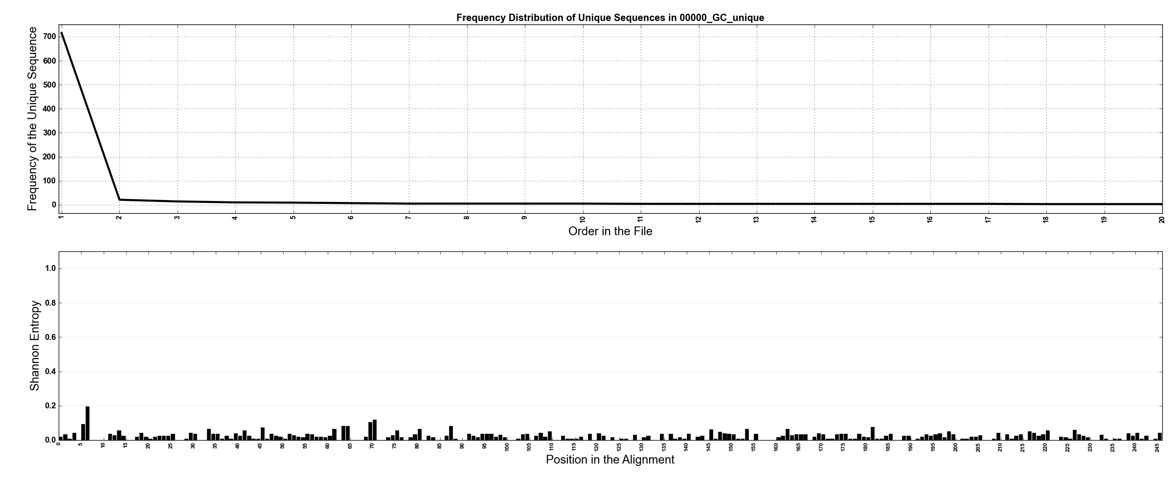
*_unique.png files: These figures are visualizations of what is going on in
*_uniquefiles. They have two panels, showing the abundance curve of unique sequences, and entropy distribution of all reads that were claimed by a given oligotype. The figure that was generated for00000_GC_uniquefile is shown below. In the top panel the abundance curve of unique sequences can be seen (according to the figure, the most abundant unique sequence comprised almost all the reads, and all others, most likely slight variations from the most abundant unique ones due to random sequencing errors, were present in very small numbers). In the bottom panel we have Shannon entropy analysis for all reads (according to the figure entropy was almost flat, which is what we would expect if all sequences in this collection do not really comprise any hidden diversity):
-
*_unique_BLAST.xml files: These XML files contain the BLAST result of the most abundant unique sequence against NCBI’s nr database. Even though it takes a lot of time to BLAST reads against nr, especially when there are many oligotypes, I find it very valuable to know if there is a perfect hit in the database for the oligotype of interest.
-
*.cPickle files: These files contain a variety of information about each oligotype in the form of serialized Python objects. They are being used by the pipeline itself to make figures and charts (see the next section).
You may also want to use a mapping file to visually investigate the similarities or dissimilarities among your samples with respect to the oligotyping resuls. Please see this article on mapping for instructions.
HTML Output
Oligotyping requires human guidance.
The best way to perform supervision is to examine results carefully, and make informed decisions about the nucleotide positions to use to explain diversity.
Luckily, the oligotyping pipeline offers an easy-to-use interface to view and examine analysis results. This is a static HTML page that is being generated by the pipeline at the end of each analysis:
oligotype mock-env-aligned.fasta mock-env-aligned.fasta-ENTROPY -c 2 -M 10
At the end of this analysis you will be given an address to visit with your favorite browser. This is a screen shot of my screen with the web address:
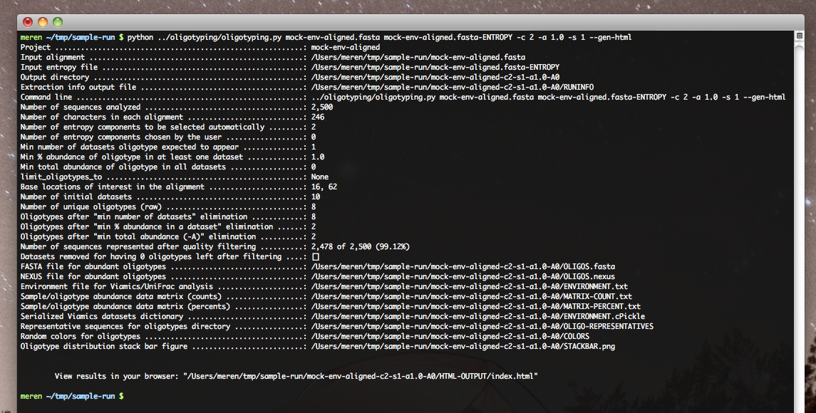
This HTML output can be seen as a summary of what analysis results show.
Since it is a static web page, you can copy it on a memory stick and carry it around, send it to your colleagues, or add as a supplementary dataset to your submission.
For instance, in order to demonstrate the results of this particular run, I copied that directory on this server:
http://oligotyping.org/sample-run/v0.96/mock-env-aligned-c2-s1-a1.0-A0-M0/HTML-OUTPUT/
In a real oligotyping analysis you will be especially interested in the ‘Oligotypes‘ section in the index page, and go through each oligotype to see whether they are converged:

Even though it looks quite uninteresting with this mock problem, it might get very sophisticated and useful when the oligotyping pipeline is dealing with real-world analyses.
Final Words
You may be wondering about the efficacy of oligotyping with actual data.
In this document I used a Pelagibacter dataset as a mock problem. It wasn’t a truly random choice. I recently analyzed 274,634 V4-V6 reads (approximately 450 nucleotides long, quality controlled and chimera checked) that were classified as Pelagibacter in a dataset that contained more than 160 samples. These 160+ samples were sequenced from environmental samples that were periodically collected from 7 geographical locations over a period of almost 2 years.
When I analyzed this data with the oligotyping pipeline explained in this document, this was the final stackbar figure, which shows the diversity within Pelagibacter (you can read the published story in the oligotyping methods paper):
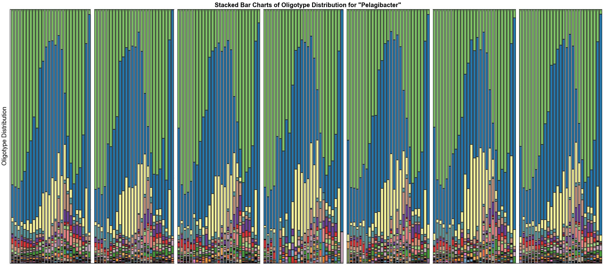
Each white bar separates one station from another. Every color represents an oligotype, and each oligotype in this figure has a perfect hit to something in NCBI with 100% sequence identity and 100% query coverage. Green and blue types in this figure are 99.6% identical. Even though they are almost identical, there is some crucial information in these sequences that is a precursor to genomic variation that affects their survival through different seasons.
This is a variation that is being missed.
When can oligotyping be useful?
I had answered that question in an earlier post in this blog:
You have 16S ribosomal RNA gene tag sequences generated from a number samples collected from various environments to investigate cross-sectional or temporal differences. After the classification (or clustering) analysis on your reads, you know the composition of your samples. There is a taxon (or an OTU) that appears to be in every sample, and you are suspecting that there is more to this taxon (or OTU) than meets the eye, you feel that there are more than one type that this unit could be broken into. Oligotyping helps you to investigate this question, and most of the time comes with surprising answers.
If you think oligotyping might be applicable to your study, and if you have questions about how to investigate your datasets via oligotyping, you can always reach me via a.murat.eren at gmail com or via @merenbey on Twitter.