


Table of Contents
Oligotyping is a supervised method, which makes it a method that welcomes its users with a learning curve. To make things a little clearer, in this article you will find the flowchart of a generic oligotyping analysis and a realistic analysis of a mock dataset. If you don’t have oligotyping pipeline installed on your system yet, there is a separate article on that topic.
Flowchart
This is a very critical statement about oligotyping:
A successful oligotyping analysis 1) identifies only those nucleotide positions necessary to explain the maximum amount of biological diversity represented by a dataset of closely related sequences, and 2) generates converged oligotypes.
Figure below illustrates a flowchart for oligotyping analysis inclusive of three critical steps (1-3) which are detailed right after the figure:
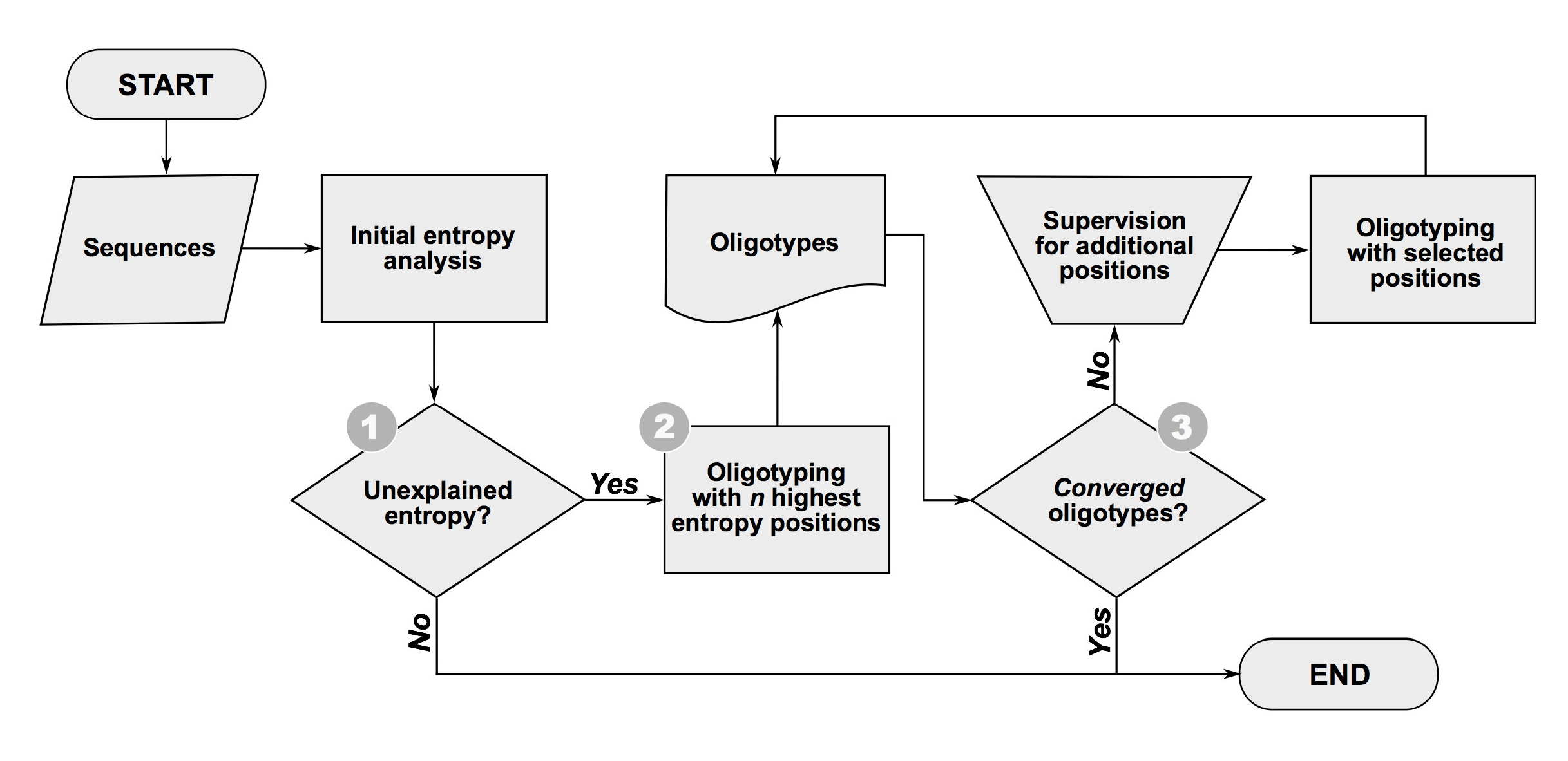
Box 1: Unexplained Entropy?
The first oligotyping step performs an initial entropy analysis on the dataset of closely related sequences to determine whether it potentially contains information for decomposing the data into distinct oligotypes. If the entropy analysis does not identify clear entropy peaks, it suggests that either all reads for the assemblage derive from one identical template that occurs in all genomes of that taxon, or the templates that give rise to distinct sequences correspond to rare genomes that cannot be confidently distinguished from random sequencing errors based on entropy values. Most sequencing errors will randomly distribute along the length of the alignment and appear as white noise that increases towards the end of the reads in entropy profiles. Our empirical observations indicate that random sequencing errors generate entropy values that hover at or below 0.2 for Illumina platforms. Therefore, if all entropy values are below 0.2 for a group of Illumina reads, oligotyping will most likely not help recover ecologically meaningful oligotypes.
Box 2: How to choose n for the initial oligotyping?
The oligotyping process should begin by setting the n parameter to select only the highest entropy positions in the first round of oligotype analysis. Setting n between 1 and 3 for the initial run is a good practiec since use of a single site will sometimes resolve multiple entropy peaks into discrete oligotypes.
Box 3: Converged oligotypes?
The decision whether to stop or continue oligotyping requires the examination of the entropy profiles of each individual oligotype recovered to make sure that the second criterion for a successful oligotyping analysis is met: all oligotypes have converged. An oligotype has converged if additional decomposition does not generate new oligotypes that exhibit differential abundances in different samples (or environments). In general, a converged oligotype will not display entropy peaks, however, there may be some high entropy positions within a converged oligotype that do not reflect ecological variation. For instance, if a microbial genome has 7 copies of the 16S rRNA gene and one varies from all others by a single nucleotide, entropy analysis will identify one potentially information-rich site that can resolve into two oligotypes with abundance ratios of 1:6 in every sample. Yet, these oligotypes will not contribute to beta diversity estimates when comparing multiple samples because the 1:6 ration is fixed by genomic content rather than differences in microbial community structures. Another case may be the existence of an entropy peak due to a homopolymer region-associated error. If remaining entropy in an oligotype appears to reflect systematic sequencing errors, the user can abort attempts to further resolve it. The oligotyping pipeline provides tools to examine the convergence of oligotypes including graphical distributions of divergent sequences in an oligotype among samples.
An example oligotyping analysis
The mock dataset we will use here to illustrate the concepts laid out in the previous section derives from a subsampling of a large publicly available human microbiome dataset. Details of this dataset are provided in Yatsunenko et al.’s 2013 paper. The subsampled dataset contains 859,302 reads that were taxonomically classified to the genus Bacteroides, and can be retrieved in FASTA format from the URL http://goo.gl/dpzJ9. To further simplify the mock dataset, reads collected from subjects from the same geographical location merged into one sample (e.g., all data collected from Malawi were merged into one sample named “Malawi”), and the final FASTA file (hereinafter called mock.fa) contained three samples: “Malawi” (53,476 reads), “Venezuela” (101,683 reads) and “USA” (704,143 reads).
The entropy profile computed for mock.fa using this command:
entropy-analysis mock.fa --quick
Figure below shows the output of the previous command. Most positions are highly conserved for all reads, hence exhibiting very low entropy values. In contrast, the large entropy peaks reveal the existence of several highly variable nucleotide positions that have the potential to identify oligotypes within the dataset.
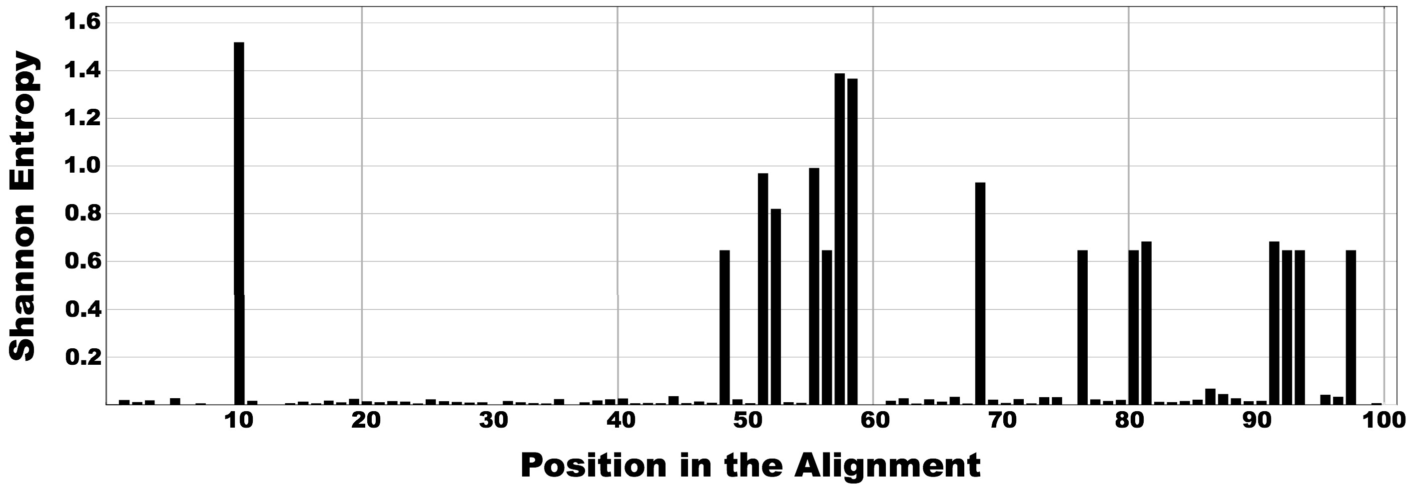
The initial round of oligotyping in this analysis set n=1 (which corresponds to Box 2 in the flowchart figure). The oligotyping pipeline will use the location of the highest entropy peak (which happens to be position 10) to generate the first round of oligotypes. The exact command to perform this operation is this:
oligotype mock.fa mock.fa-ENTROPY -c 1 -M 50
where mock.fa-ENTROPY is the file that was generated after the initial entropy analysis. -M is the minimum substantive abundance parameter. You may see the Methods section in the oligotyping manuscript for the detailed explanation for it, but In briefly, it is for noise removal and tells the pipeline to eliminate any oligotype in which the frequency of the most abundant unique sequence is below -M.
Oligotyping analysis of mock.fa using the highest entropy location, position 10, identifies 3 oligotypes: C (383,788 reads), G (297,937 reads) and T (177,577 reads). The HTML output for this analysis can be viewed using the web address http://goo.gl/oY8dD (please visit this link and follow the steps described here using the analysis results provided). Figure below shows the distribution profiles of these oligotypes among three samples:

Each oligotype shown in this figure is composed of reads from the mock dataset that possessed the same nucleotide at the 10th position. Naturally, the entropy is zero at the 10th location of each individual oligotype following the first round of oligotyping. As the figure indicates, some of the diversity of Bacteroides reads is already explained by the oligotypes.
The decision to stop or continue oligotyping brings us to the second criterion for a successful oligotyping analysis: determining whether the oligotypes have converged. Figure below displays entropy profiles of oligotype C, G and T (abundance curves can also be seen in the HTML output):
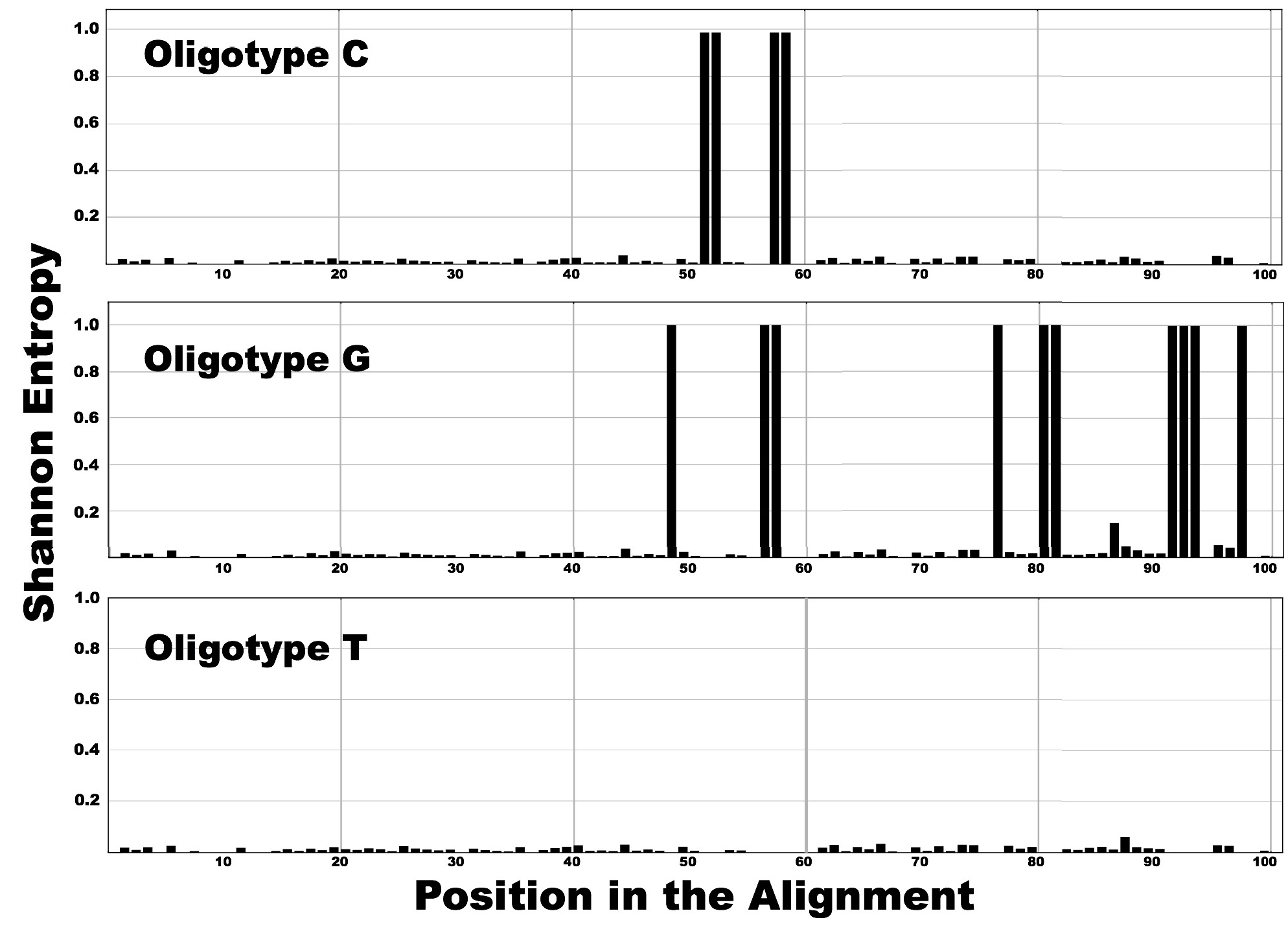
You can see that the oligotype T has minimal entropy (remains below 0.1), which indicates very little variance for all positions across all reads for this oligotype. In contrast, oligotypes C and G exhibit numerous entropy peaks, which indicate that the oligotyping analysis should continue with additional nucleotide positions (along with the previously selected 10th position).
The pipeline’s output for oligotype C (http://goo.gl/50Ihp) reveals additional peaks with similar entropy values at the 51st, 52nd, 57th and 58th positions. Their information content should be equally efficient for resolving the diversity confined in oligotype C. Under this condition, the pipeline facilitates user decisions about site selection for subsequent rounds of oligotyping. For example, the proximal location relative to the start of a sequencing read where quality tends to be high would favor the selection of the 51st site in combination with the 10th position for identifying a new oligotype. The next round of oligotyping could start with 51th and 10th positions. However, the entropy profiles of the remaining first-round oligotypes (in this example, oligotype G) can reveal high entropy sites that are shared among oligotypes and facilitate the convergence of oligotypes with the use of minimal number of additional nucleotide positions.
Oligotype G’s entropy profile (http://goo.gl/ps0LS) reveals that the 48th, 56th, 57th, 76th, 80th, 81st, 91st, 92nd, 93rd and 97th positions exhibit variation and hence information content that can further explain the diversity confined in this oligotype. Similar to the case of oligotype C, the 48th position (closest to the beginning of the alignment) might further partition oligotype G. However, the candidate sites in both oligotypes C and G include the 57th position (see Fig. S8). By using this site, the analysis will require only two positions (10th and 57th), instead of three (10th, 51st and 48th) in the second round of oligotyping. To obtain further resolution using the 10th and 57th positions to partition the sequence alignment mock.fa, the second round of oligotyping in this example run by this command:
oligotype mock.fa mock.fa-ENTROPY -C 10,57 -M 50
Note the use of -C followed by the comma separated list of chosen locations, instead of -c used in the first round followed by the number of maximum entropy locations.
Oligotyping analysis of mock.fa using the two entropy locations identified in a supervised manner results in 5 oligotypes: CA (219,745 reads), TT (177,577 reads), CT (164,043 reads), GT (155,970 reads) and GC (141,967 reads). The HTML output of the analysis can be viewed using the web address http://goo.gl/aMleb. Figure below shows the updated distribution profiles of these oligotypes among three samples:
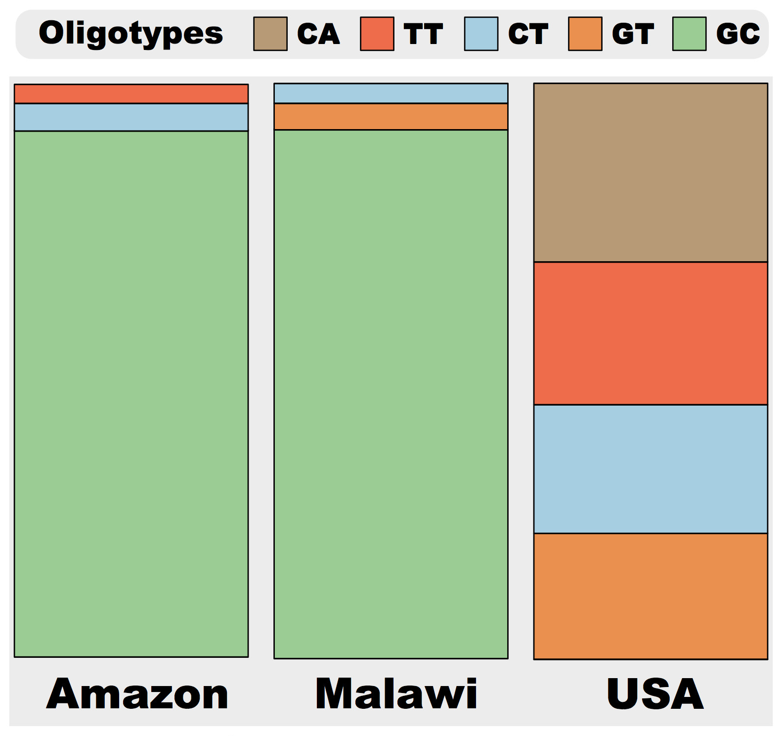
Compared to the previous stackbarchart figure, new result shows increased separation of the USA sample from Amazon and Malawi samples. The greater dissimilarity comes from the division of oligotype G, which was shared between all three samples at the end of the first oligotyping run based on 10th position alone, into two oligotypes GC and GT with the addition of the 57th position to the second round of oligotyping. Now oligotype G partitions into an Amazon and Malawi specific oligotype GC, and another oligotype GT, that is more abundant in the USA sample.
As in the previous round of oligotyping, the decision of whether to stop or continue oligotyping requires evaluation of oligotype convergence by the examination of the entropy profiles of each individual oligotype. See Figure below shows entropy profiles of oligotype CA, TT, CT, GT and GC.

All oligotypes, with the exception of GT, are fully resolved. Oligotype GT has one entropy peak that coincides with the 86th location. Another round of oligotyping that includes the 86th location to the previous two locations could further resolve oligotype GT. Yet, when we examine the divergent sequence distribution profiles within this oligotype (profiles can be seen at the web address http://goo.gl/Zr3OG), we conclude that further decomposition of oligotype GT does not improve the resolution of beta diversity and thus oligotyping should end after round 2.
With this decision, oligotyping of mock.fa process concludes with an improved, ecologically meaningful dissection of the diversity of Bacteroides organisms in this dataset.