The Prochlorococcus metapangenome
Table of Contents
- Linking pangenomes and metagenomes: the Prochlorococcus metapangenome.
- Downloading the 31 Prochlorococcus isolate genomes
- Downloading the 93 TARA Oceans metagenomes
- Metagenomic read recruitment using the genomes
- Profiling the mapping results with anvi’o
- Generating a merged anvi’o profile database
- Generating a collection
- Niche partitioning of genomes
- Classification of genes as ECGs and EAGs by the distribution of genes in a genome across metagenomes
- Environmental connectivity of each gene cluster
This reproducible bioinformatics workflow describes program names and exact parameters we used throughout every step of the analysis of 31 Prochlorococcus isolate genomes and 93 TARA Oceans metagenomes, which relied predominantly on the open-source analysis platform anvi’o in the following study:
Linking pangenomes and metagenomes: the Prochlorococcus metapangenome.

- Metapangenomes reveal to what extent genes that may be linked to the ecology and fitness of microbes are conserved within a phylogenetic clade.
- Reproducible bioinformatics workflow.

Please find the published study along with its review history here: https://peerj.com/articles/4320/
All anvi’o analyses in this document are performed using the anvi’o version v3 (but it is OK to use anything newer than that, although pelase don’t forget to run anvi-migrate-db on your databases). Please see the installation notes to download the appropriate version through PyPI, Docker, or GitHub.
All public data items used and produced by this study is deposited here.
While our study was in review, we decided to stop using ‘protein clusters’ and start using ‘gene clusters’ to describe what comes from the other end of pangenomic analyses. Our reasons and resolution, as well as other opinions around this topic are detailed here. If you see ‘protein clusters’ in some of our output file names, please don’t be alarmed. Starting with anvi’o v4, the terminology will be much cleaner. The same things goes for ‘environmentally connected/disconnected genes’ (ECGs and EDGs). We now call them ‘environmental core/accessory genes’ (ECGs and EAGs). The definition of these terms and why we needed these acronyms are explained in our manuscript and in this document, but if you see EDGs in some output files, please remember that they will all be EAGs starting with v4. We apologize for all the inconvenience.
The URL https://merenlab.org/data/prochlorococcus-metapangenome serves the most up-to-date version of this document.
Summary
In this study,
-
We generated an anvi’o contigs database describing 31 Prochlorococcus isolate genomes.
-
Using isolate genomes recruited reads from TARA Oceans Project metagenomes and profiled recruitment results,
-
Characterized the pangenome of the isolates genomes,
-
Linked the pangenome with metagenomes.
Sections in this document will detail all the steps of downloading and processing Prochlorococcus isolate genomes and TARA Oceans Project metagenomes, mapping metagenomic reads onto the Prochlorococcus isolate genomes, computing the Prochlorococcus pangenome, and finally creating a metapangenome by linking the pangenome to the environment.
Please feel free to leave a comment, or send an e-mail to us if you have any questions.
Setting the stage
This section explains how to download a set of 31 Prochlorococcus isolate genomes and download and quality filter short metagenomic reads from the TARA Oceans project (Sunagawa et al., 2015).
The TARA Oceans metagenomes we analyzed are publicly available through the European Bioinformatics Institute (EBI) repository and NCBI under project IDs ERP001736 and PRJEB1787, respectively.
Downloading the 31 Prochlorococcus isolate genomes
You can get a copy of the FASTA file containing all 31 Prochlorococcus isolate genomes (and the 74 Prochlorococcus SAGs incorporated in the study) into your working directory using these commands:
curl -L https://ndownloader.figshare.com/files/9416614 \
     -H "User-Agent: Chrome/115.0.0.0" \
     -o PROCHLOROCOCCUS-FASTA-FILES.tar.gz
tar -xzvf PROCHLOROCOCCUS-FASTA-FILES.tar.gz
Downloading the 93 TARA Oceans metagenomes
We described these steps in this workflow document for another study. Please click to that link, follow the instructions starting from the section “Downloading the TARA Oceans metagenomes”, and come back to this document once you reached to the section “Co-assembling metagenomic sets” (so all you do is to download metagenomes and perform quality filtering).
Generating an anvi’o contigs database
We used the program anvi-gen-contigs-database with default parameters to profile all contigs for Prochlorococcus isolate genomes, and generate an anvi’o contigs database that stores for each contig the DNA sequence, GC-content, tetranucleotide frequency, and open reading frames as Prodigal v2.6.3 (Hyatt et al., 2010) identifies them:
anvi-gen-contigs-database -f Prochlorococcus-isolates.fa \
                          -o Prochlorococcus-CONTIGS.db \
                          -n "Prochlorococcus isolate genomes"
We then used the program anvi-run-hmms to identify archaeal and bacterial single-copy core genes (SCGs) in Prochlorococcus isolates:
anvi-run-hmms -c Prochlorococcus-CONTIGS.db \
              --num-threads 20
This step uses HMMER v3.1b2 (Eddy, 2011) to match genes to previously determined HMM profiles for bacterial and archaeal SCGs by Campbell et al and Rinke et al.
We finally used the program anvi-run-ncbi-cogs to search the NCBI’s Clusters of Orthologous Groups (COGs) to assign functions to genes in our contigs database:
anvi-run-ncbi-cogs -c Prochlorococcus-CONTIGS.db \
                   --num-threads 20
Results of this step is used to display gene clusters with known functions in the interactive interface for our downstream pangenomic analysis, and the summary outputs.
doi:10.6084/m9.figshare.5447224 serves the resulting anvi’o contigs database.
Recruiting and profiling reads form metagenomes
This section explains various steps to characterize the occurrence of each Prochlorococcus genome and individual gene in TARA Oceans metagenomes.
Metagenomic read recruitment using the genomes
The recruitment of metagenomic reads is commonly used to assess the coverage of contigs, which provides the essential information that is employed by anvi’o to assess the relative distribution of genomes across metagenomes.
We mapped short reads from the 93 TARA Oceans metagenomes onto the contigs contained in Prochlorococcus-isolates.fa using Bowtie2 v2.0.5 (Langmead and Salzberg, 2012). We stored the recruited reads as BAM files using samtools (Li et al., 2009).
We first built a Bowtie2 database for Prochlorococcus-isolates.fa:
bowtie2-build Prochlorococcus-isolates.fa Prochlorococcus-isolates
We then mapped each metagenome against the contigs contained in Prochlorococcus-isolates.fa (you must have the samples.txt in your directory if you followed the download instructions for metagenomes from the other workflow, if you didn’t, this file simply describes the read 1 and read 2 for each metagenomic sample):
for sample in `awk '{print $1}' samples.txt`
do
    if [ "$sample" == "sample" ]; then continue; fi
    # do the bowtie mapping to get the SAM file:
    bowtie2 --threads 20 \
            -x Prochlorococcus-isolates \
            -1 $sample-QUALITY_PASSED_R1.fastq.gz \
            -2 $sample-QUALITY_PASSED_R2.fastq.gz \
            --no-unal \
            -S $sample.sam

    # covert the resulting SAM file to a BAM file:
    samtools view -F 4 -bS $sample.sam > $sample-RAW.bam

    # sort and index the BAM file:
    samtools sort $sample-RAW.bam -o $sample.bam
    samtools index $sample.bam

    # remove temporary files:
    rm $sample.sam $sample-RAW.bam
done
This process has resulted in 93 sorted and indexed BAM files that describe the mapping of more than 30 billion short reads to contigs contained in the FASTA file Prochlorococcus-isolates.fa.
Profiling the mapping results with anvi’o
After recruiting metagenomic short reads using contigs stored in the anvi’o contigs database for Prochlorococcus genomes, we used the program anvi-profile to process the BAM files and to generate anvi’o profile databases that contain the coverage and detection statistics of each Prochlorococcus contig in a given metagenome:
for sample in `awk '{print $1}' samples.txt`
do
    if [ "$sample" == "sample" ]; then continue; fi

    anvi-profile -c Prochlorococcus-CONTIGS.db \
                 -i $sample.bam \
                 -M 100 \
                 --skip-SNV-profiling \
                 --num-threads 16 \
                 -o $sample
done
Please read the following article for parallelization of anvi’o profiling (details of which can be important to consider especially if you are planning to send it to a cluster): The new anvi’o BAM profiler.
Generating a merged anvi’o profile database
Once the individual PROFILE databases were generated, we used the program anvi-merge to generate a merged anvi’o profile database:
anvi-merge */PROFILE.db \
           -o Prochlorococcus-MERGED \
           -c Prochlorococcus-CONTIGS.db
The resulting merged profile database describes the coverage and detection statistics for each contig across all 93 metagenomes.
doi:10.6084/m9.figshare.5447224 serves the merged anvi’o merged profile.
Generating a collection
At this point anvi’o still doesn’t know how to link contigs to each isolate genome. In anvi’o, this kind of knowledge is maintained through ‘collections’. In order to link contigs to genomes of origin, we used the program anvi-import-collection to create an anvi’o collection in our merged profile database.
We first generated a 2-columns, TAB-delimited collections file:
for split_name in `sqlite3 Prochlorococcus-CONTIGS.db 'select split from splits_basic_info;'`
do
    # in this loop $split_name looks like this AS9601-00000001_split_00001, form which
    # we can extract the genome name the split belongs to:
    GENOME=`echo $split_name | awk 'BEGIN{FS="-"}{print $1}'`

    # print it out with a TAB character
    echo -e "$split_name\t$GENOME"
done > Prochlorococcus-GENOME-COLLECTION.txt
The resulting file Prochlorococcus-GENOME-COLLECTION.txt looked like this:
$ head Prochlorococcus-GENOME-COLLECTION.txt
AS9601-00000001_split_00001 AS9601
AS9601-00000001_split_00002 AS9601
AS9601-00000001_split_00003 AS9601
AS9601-00000001_split_00004 AS9601
AS9601-00000001_split_00005 AS9601
AS9601-00000001_split_00006 AS9601
AS9601-00000001_split_00007 AS9601
AS9601-00000001_split_00008 AS9601
AS9601-00000001_split_00009 AS9601
AS9601-00000001_split_00010 AS9601
(...)
So each contig name is listed in the first column, and the genome they belonged is listed in the second.
The file Prochlorococcus-GENOME-COLLECTION.txt is also available here.
We then used the program anvi-import-collection to import this collection into the anvi’o profile database by naming this collection Genomes, so anvi’o knows about this:
anvi-import-collection Prochlorococcus-GENOME-COLLECTION.txt \
                       -c Prochlorococcus-CONTIGS.db \
                       -p Prochlorococcus-MERGED/PROFILE.db \
                       -C Genomes
We then double-checked whether we had a collectin called ‘Genomes’ using anvi-show-collections-and-bins:
anvi-show-collections-and-bins -p PROFILE.db

Collection: "Genomes"
===============================================
Collection ID ................................: Genomes
Number of bins ...............................: 31
Number of splits described ...................: 2,671
Bin names ....................................: AS9601, CCMP1375, EQPAC1, GP2,
LG, MED4, MIT9107, MIT9116, MIT9123, MIT9201, MIT9202, MIT9211, MIT9215, MIT9301,
MIT9302, MIT9303, MIT9311, MIT9312, MIT9313, MIT9314, MIT9321, MIT9322, MIT9401,
MIT9515, NATL1A, NATL2A, PAC1, SB, SS2, SS35, SS51
Since everything looks good, we summarized this collection to create a tables with gene coverage values across metagenomes per genome:
anvi-summarize -c Prochlorococcus-CONTIGS.db \
               -p Prochlorococcus-MERGED/PROFILE.db \
               -C Genomes \
               --init-gene-coverages \
               -o Prochlorococcus-SUMMARY
This summary contains all key information regarding the occurrence of genomes in metagenomes that will be relevant to investigate the niche partitioning of genomes.
You can find the summary output directory (which is a static HTML output that can be displayed without an anvi’o installation by double-clicking the index.html file) in the archive served at the url doi:10.6084/m9.figshare.5447224.
Computing the Prochlorococcus pangenome
To generate the Prochlorococcus pangenome, and to visuaize it, we used the anvi’o programs anvi-gen-genomes-storage, anvi-pan-genome, and anvi-display-pan on the following order.
We first created the file internal-genomes.txt so the pangenomic workflow can access to all the genomes the information about which are stored in the Genomes collection in the merged profile database individually (details of the anvi’o pangenomic workflow are here). The internal genomes file can be downloaded using this command:
wget http://merenlab.org/data/prochlorococcus-metapangenome/files/internal-genomes.txt
And here is how it looks like:
$ head internal-genomes.txt
name     bin_id   collection_id  profile_db_path                    contigs_db_path
MIT9322  MIT9322  Genomes        Prochlorococcus-MERGED/PROFILE.db  Prochlorococcus-CONTIGS.db
MIT9321  MIT9321  Genomes        Prochlorococcus-MERGED/PROFILE.db  Prochlorococcus-CONTIGS.db
MED4     MED4     Genomes        Prochlorococcus-MERGED/PROFILE.db  Prochlorococcus-CONTIGS.db
MIT9301  MIT9301  Genomes        Prochlorococcus-MERGED/PROFILE.db  Prochlorococcus-CONTIGS.db
MIT9303  MIT9303  Genomes        Prochlorococcus-MERGED/PROFILE.db  Prochlorococcus-CONTIGS.db
SS2      SS2      Genomes        Prochlorococcus-MERGED/PROFILE.db  Prochlorococcus-CONTIGS.db
AS9601   AS9601   Genomes        Prochlorococcus-MERGED/PROFILE.db  Prochlorococcus-CONTIGS.db
MIT9211  MIT9211  Genomes        Prochlorococcus-MERGED/PROFILE.db  Prochlorococcus-CONTIGS.db
Using this configuration, we generated a genomes storage,
anvi-gen-genomes-storage -i internal-genomes.txt \
                         -o Prochlorococcus-PAN-GENOMES.db
Computed the pangenome,
anvi-pan-genome -g Prochlorococcus-PAN-GENOMES.db \
                --use-ncbi-blast \
                --minbit 0.5 \
                --mcl-inflation 10 \
                --project-name Prochlorococcus-PAN \
                --num-threads 20
and visualized it:
anvi-display-pan -p Prochlorococcus-PAN/Prochlorococcus-PAN-PAN.db \
                 -s Prochlorococcus-PAN/Prochlorococcus-PAN-SAMPLES.db \
                 -g Prochlorococcus-GENOMES.db
So far so good? Good.
From the interface, we selected our bins of interest:
-
HL+LL core: gene clusters detected in all 31 genomes
-
HL core: gene clusters only detected in all HL clade genomes
-
LL core: gene clusters only detected in all LL clade genomes
-
SINGLETONS: gene clusters only detected in one genome
We then saved them as a collection named default. We finally summarized the Prochlorococcus pangenome using the program anvi-summarize:
anvi-summarize -p Prochlorococcus-PAN/Prochlorococcus-PAN-PAN.db \
               -g Prochlorococcus-GENOMES.db \
               -C default \
               -o Prochlorococcus-PAN-SUMMARY
The resulting summary folder contains the file Prochlorococcus-PAN_protein_clusters_summary.txt that links each gene to gene clusters, genomes, functions, and bins selected from the interface.
The metapangenome: Linking the pangenome to the environment
Just to make sure we are on the same page, here is a definition: we define ‘metapangenome’ as the outcome of the analysis of pangenomes in conjunction with the environment where the abundance and prevalence of gene clusters and genomes are recovered through shotgun metagenomes.
Niche partitioning of genomes
The anvi’o metagenomic summary output described in the previous section contains infomration to identify relative distribution of each genome across the 93 metagenomes.
We created a text file, Prochlorococcus-METAGENOME-samples-information.txt (available here) to display the relative abundance of genomes across samples, and we extended this file with various information such as the phlogenetic clade membership of each genome. Using this file together with the file Prochlorococcus-PAN-samples-order.txt (one of the default outputs of anvi-pan-genome step), we generated an anvi’o samples database:
anvi-gen-samples-info-database -D Prochlorococcus-METAGENOME-samples-information.txt \
                               -R Prochlorococcus-PAN/Prochlorococcus-PAN-samples-order.txt \
                               -o Prochlorococcus-METAPAN-SAMPLES.db
The file Prochlorococcus-METAPAN-SAMPLES.db is similar to the file Prochlorococcus-PAN-SAMPLES.db automatically generated by anvi’o, except it contains extra information for each genome.
Classification of genes as ECGs and EAGs by the distribution of genes in a genome across metagenomes
Assuming the environmental ‘niche’ of a population is defined by the metagenomes in which it is ‘detected’, here we define ‘environmental core genes’ of a population as the genes that are systematically detected in its ‘niche’. In contrast, the genes that are not systematically detected within the niche of a given population represent its ‘environmental accessory genes’. Genes in a population that are classified as ‘environmental core’ given metagenomic data can be classified as ‘accessory’ given a pangenome, and vice versa. So, to avoid any confusion between these operationally distinct class designations, we refer to the genes classified given the metagenomic data as the ‘environmental core genes’ (ECGs) and the ‘environmental accessory genes’ (EAGs).
This section is just a bonus, and you can skip to the next section unless you are interested in seeing how did we generate this figure, where you can see the distribution of genes in a single genome across a set of metagenomes:
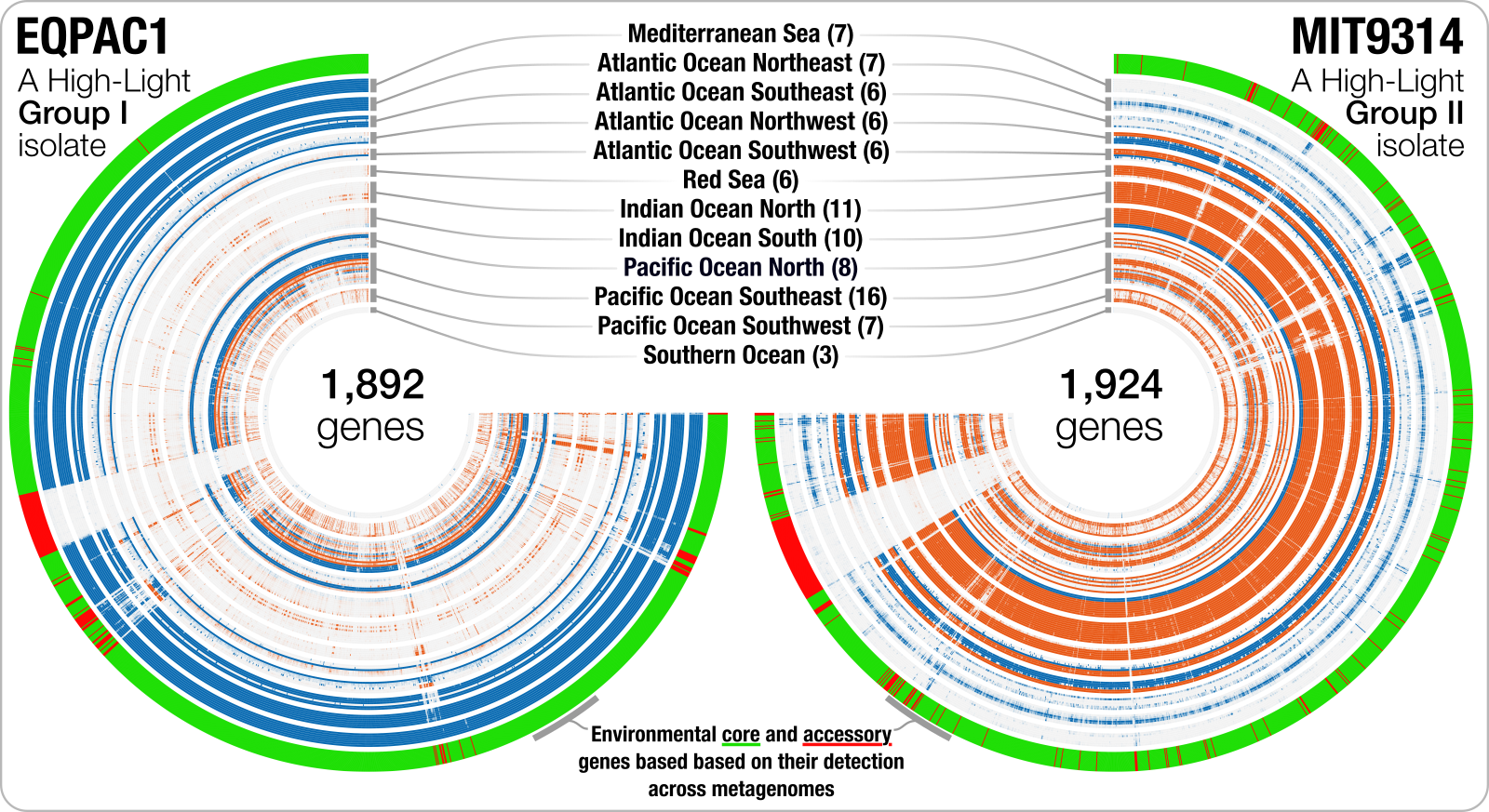
In this figure, each layer is a metagenome, and each leaf represents a gene ordered by synteny. The outer layer indicates which ones are systemmatically occurring across metagenomes, and which ones are not. Although this step is not necessary, it is important to see and better understand where the data we will be working with in the next chapter is coming from.
Basically at this point we have a merged anvi’o profile database that keeps the coverage information per genome per gene across all metagenomes. Incidentally, we also have an anvi’o program that can generate some output files that can help us to visualize the distribution of ‘each gene’ (not each contig as we usually do) across metagenomes in a given ‘bin’. For instance, to export this data for EQPAC1 and MIT9314, one could run this anvi’o program the following way:
# generate gene-level distribution data for MIT9314:
anvi-script-gen-distribution-of-genes-in-a-bin -p Prochlorococcus-MERGED/PROFILE.db \
                                               -c Prochlorococcus-CONTIGS.db \
                                               -C Genomes \
                                               --fraction-of-median-coverage 0.25 \
                                               -b MIT9314 \
                                               -o MIT9314-ENV-DETECTION.txt


# do the same for EQPAC1:
anvi-script-gen-distribution-of-genes-in-a-bin -p Prochlorococcus-MERGED/PROFILE.db \
                                               -c Prochlorococcus-CONTIGS.db \
                                               -C Genomes \
                                               --fraction-of-median-coverage 0.25 \
                                               -b EQPAC1 \
                                               -o EQPAC1-ENV-DETECTION.txt
These will generate multiple output files for both bins. The file that ends with -ENV-COVs.txt will be a TAB-delimited matrix with gene coverage values across each sample for the a given bin. In contrast, the file that ends with -ENV-DETECTION.txt will be an additional data file for the anvi-interactive to show which genes did occur systemmatically across metagenomes given the ‘fraction of median coverage’ criterion.
For instance, you can download the output files for MIT9314 the following way:
wget http://merenlab.org/data/prochlorococcus-metapangenome/files/MIT9314-GENE-COVs.txt
wget http://merenlab.org/data/prochlorococcus-metapangenome/files/MIT9314-ENV-DETECTION.txt
And run the interactive interace to display the distribution of genes that appears in the first panel in the figure above:
anvi-interactive -d MIT9314-GENE-COVs.txt \
                 -A MIT9314-ENV-DETECTION.txt \
                 --manual \
                 -p GENES-PROFILE.db \
                 --title "Prochlorococcus MIT9314 genes across TARA Oceans Project metagenomes"
If you run the command above successfully, and clicked ‘Draw’ in the interace, you must already have realized that the colors used in the figure is not be there, but if you like, you can download the following state file, import it into the profile database GENES-PROFILE.db anvi’o just generated for you, and re-run the interactive interface:
# download the state file:
wget http://merenlab.org/data/prochlorococcus-metapangenome/files/GENES-PROFILE.json

# import it into the db
anvi-import-state -s GENES-PROFILE.json \
                  -p GENES-PROFILE.db \
                  -n default

# re-run the interactive interface:
anvi-interactive -d MIT9314-GENE-COVs.txt \
                 -A MIT9314-ENV-DETECTION.txt \
                 --manual \
                 -p GENES-PROFILE.db \
                 --title "Prochlorococcus MIT9314 genes across TARA Oceans Project metagenomes"
This time it should be looking just like the figure, prior to polishing, of course.
In the next chapter, we in fact will generate a single file that summarizes detection statistics for each gene in each genome across each metagenome, which will give us an idea about the ratio of systemmatically occurring and systemmatically missing genes in our gene clusters.
Environmental connectivity of each gene cluster
Most these steps are specific to anvi’o v3 and have been imporoved so dramatically. If you are struggling with a similar analysis using later versions of anvi’o and our online tutorials do not seem to help, please let us know and we will help you sort things out.
The next step is to link each gene from each genome across every metagenome to characterize the ratio of environmentally accessory genes (EAGs) to environmentally core genes (ECGs) in each gene cluster in the pangenome. This way, we will be linking the pangenome to the environment not only through the distribution statistics of each genome across each metagenome (see ‘Niche partitioning of genomes’), but also by connecting the contents of each gene cluster to the environment:
anvi-script-gen-environmental-core-summary -i internal-genomes.txt \
                                           -p Prochlorococcus-PAN/Prochlorococcus-PAN-PAN.db \
                                           -g Prochlorococcus-GENOMES.db \
                                           --fraction-of-median-coverage 0.25 \
                                           -O ENVIRONMENTAL-CORE
The program will result in two files. ENVIRONMENTAL-CORE.txt, and ENVIRONMENTAL-CORE-GENES.txt. The latter is simply a resource to go back to the classification of each gene in each genome regarding whether they were systemmatically occurring across meatgenomes. In contrast, the file ENVIRONMENTAL-CORE.txt is the primary output file to visualize the detection statistics of the contents of the gene clusters given the environmental data. The content of this file will look like this, where each line will show the number of genes in each cluster based on their membership in one of the three classes:
$ head ENVIRONMENTAL-CORE.txt
pc_name	Detection!EDG;ECG;NA
PC_00003005	4;0;0
PC_00001555	0;5;13
PC_00006377	0;0;1
PC_00000393	0;25;6
PC_00006445	1;0;0
PC_00003323	0;3;0
PC_00005579	0;1;0
PC_00006152	0;0;1
PC_00000668	0;25;6
When we provide this file as an additional data to the program anvi-display-pan, its contents will be visualized as ‘bar plots’ by anvi’o interactive interface:
anvi-display-pan -p Prochlorococcus-PAN/Prochlorococcus-PAN-PAN.db \
                 -s Prochlorococcus-METAPAN-SAMPLES.db \
                 -g Prochlorococcus-GENOMES.db \
                 -A ENVIRONMENTAL-CORE.txt \
                 --title "Prochlorococcus Metapangenome"
Which should a more primitive version of this:
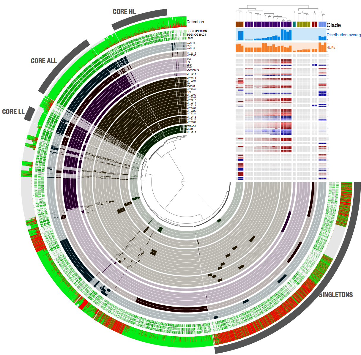
In fact, the resulting display is publicly available on the anvi’server and you can interactively visualize a copy of it here:
https://anvi-server.org/merenlab/prochlorococcus_metapangenome
doi:10.6084/m9.figshare.5447227 serves the anvi’o files for the Prochlorococcus metapangenome.
Migrating your databases
If you are using an anvi’o version newer than v3 and wish you visualize the metapangenome above, you will need to migrate the databases to your new version of anvi’o. Fortunately it is qutie simple. Please run the commands below one by one in the directory after unpacking the file you have downloaded:
# migrate the pan database
ANVIO_SAMPLES_DB=Prochlorococcus-METAPAN-SAMPLES.db anvi-migrate-db Prochlorococcus-PAN-PAN.db

# migrate the genomes storage
anvi-migrate-db Prochlorococcus-GENOMES.db

# convert the additional layers to the new format
echo -e "pc_name\tDetection#EDG\tDetection#ECG\tDetection#NA" | sed 's/#/!/g' > ENVIRONMENTAL-CORE-FIXED.txt
grep -v 'pc_name' ENVIRONMENTAL-CORE.txt | awk 'BEGIN{FS=";"}{print $1 "\t" $2 "\t" $3}' >> ENVIRONMENTAL-CORE-FIXED.txt

# import additional layers into the pan database
anvi-import-misc-data -t items ENVIRONMENTAL-CORE-FIXED.txt -p Prochlorococcus-PAN-PAN.db

# remove garbage
rm -rf *SAMPLES* ENVIRONMENTAL-CORE.txt 00_run.sh ENVIRONMENTAL-CORE-GENES.txt

# finally, visualize, and say *tada*
anvi-display-pan -p Prochlorococcus-PAN-PAN.db -g Prochlorococcus-GENOMES.db
Please let us know if you run any trouble with any of these :)
If you’ve gone through the entire document, we thank you for your time and interest. If you have any questions, or if you would like any part of this document to be clarified, please leave a comment.
References
-
Eddy SR. (2011). Accelerated Profile HMM Searches. PLoS Comput Biol 7: e1002195.
-
Eren AM, Esen ÖC, Quince C, Vineis JH, Morrison HG, Sogin ML, et al. (2015). Anvi’o: an advanced analysis and visualization platform for ‘omics data. PeerJ 3: e1319.
-
Eren AM, Vineis JH, Morrison HG, Sogin ML. (2013). A Filtering Method to Generate High Quality Short Reads Using Illumina Paired-End Technology. PLoS One 8: e66643.
-
Hyatt D, Chen G-L, Locascio PF, Land ML, Larimer FW, Hauser LJ. (2010). Prodigal: prokaryotic gene recognition and translation initiation site identification. BMC Bioinformatics 11: 119.
-
Langmead B, Salzberg SL. (2012). Fast gapped-read alignment with Bowtie 2. Nat Methods 9: 357–359.
-
Li H, Handsaker B, Wysoker A, Fennell T, Ruan J, Homer N, et al. (2009). The Sequence Alignment/Map format and SAMtools. Bioinformatics 25: 2078–2079.
-
Minoche AE, Dohm JC, Himmelbauer H. (2011). Evaluation of genomic high-throughput sequencing data generated on Illumina HiSeq and genome analyzer systems. Genome Biol 12: R112.
-
Sunagawa S, Coelho LP, Chaffron S, Kultima JR, Labadie K, Salazar G, et al. (2015). Ocean plankton. Structure and function of the global ocean microbiome. Science 348: 1261359.