DWH O. desum v2: Most abundant Oceanospirillaceae population in the Deepwater Horizon Oil Plume

During the Deepwater Horizon oil spill in the Gulf of Mexico in 2010, about half of the leaked oil did not reach the surface and instad formed a ‘plume’ in deep sea. Multiple studies have shown that microorganisms affiliated to a single bacterial lineage (within the family Oceanospirillaceae) dominated the oil plume soon after this major environmental disaster started.

These microorganisms have not been isolated but three large metagenomes have been generated directly from oil plume samples and the surrounding water by Mason et al. (2012), providing an opportunity to study the genomic content of populations dominating this environment.

Using CLC for metagenomic assembly, and anvi’o for binning and curation, we first characterized a highly fragmented and incomplete population genome from the co-assembly of these metagenomes (Eren et al., 2015). We named this 1.07 Mbp long and 58.3% complete population genome DWH Oceanospirillaceae Desum (or DWH O. Desum, with an unknwon genus name), and claimed it represented the most abundant bacterial population in the plume.

More recently, DWH O. Desum was at the heart of a little exchange in PNAS, which motivated us to get a better population genome using a newer assembly algorithm, since things have changed a lot since 2015. After performing both co-assemblies and single assemblies using multiple metagenomic assemblers, we selected one workflow that allowed us to recover a population genome of DWH O. desum with substantially improved quality: metaSPAdes assembly of the Distal metagenome, followd by binning and curation with anvi’o.

The remaining of this blog post will describe our semi-reproducible workflow and general trends of the population genome that once dominated the oil plume.

It is only ‘semi-reproducible’, becaue it assumes you have the metagenomic short reads from distal, proximal, and control sites published in Mason et al. in your work directory. If someone ever needs a fully reproducible version of this workflow, and feel too lazy to download the metagenomes themselves, they should e-mail Meren, and he will make available compressed archives for short reads.

Summary and citable DOIs

You can download a copy of DWH O. desum v2 (a 2.81 Mbp long, 97.1% complete and 0% redundant near-complete population genome), and cite it in your work through this DOI:

FASTA file for DWH O. Desum: doi:10.6084/m9.figshare.5633344

You can download the anvi’o contigs database and the merged profile database here:

Anvi’o files for DWH O. Desum: doi:10.6084/m9.figshare.5633347

Contents of the package above is the result of the workflow detailed in the rest of this post. It simply gives you acceess to the read recruitment results from three oil spill metagenomes that are used to recover the population genome among other sweets.

Analyzing a metaSPAdes assembly of the Distal metagenome

We analyzed the metaSPAdes assembly output and the mapped reads altogether using the metagenomic workflow of anvi’o v2.4.0 (the entire analysis took about 2 days).

What follows is a brief summary of our reproducible workflow.

The assembly

metaspades.py -1 DISTAL-METAGENOME_R1.fastq \
              -2 DISTAL-METAGENOME_R2.fastq \
              --threads 20 \
              -o OUTPUT

The file OUTPUT/scaffolds.fasta contains scaffolds metaSPAdes generated.

Generating an anvi’o contigs database

Both the tetra-nucleotide frequency and differential mean coverage of scaffolds across metagenomes are instrumental to accurate binning of scaffolds into metagenomic bins.

To prepare for the binning step, we first removed scaffolds too short to produce a reliable tetra-nucleotide frequency using the program anvi-script-reformat-fasta, and then used the program anvi-gen-contigs-database with default parameters to profile all scaffolds and generate an anvi’o contigs database that stores the nucleic acid sequence, tetra-nucleotide frequency, GC-content, and the coordinates of genes Prodigal v2.6.3 (Hyatt et al., 2010) identified:

anvi-script-reformat-fasta OUTPUT/scaffolds.fasta \
                           --simplify-names \
                           --prefix OIL_PLUME \
                           --min-len 1000 \
                           --report-file names-report.txt \
                           -o ASSEMBLY-1K.fa

This created a FASTA file, ASSEMBLY-1K.fa, containing 6,123 scaffolds longer than 1,000 nt, from which, we generated an anvi’o contigs database:

anvi-gen-contigs-database -f ASSEMBLY-1K.fa \
                          -o CONTIGS.db

Identifying single-copy core genes in scaffolds

We used the program anvi-run-hmms to identify genes in the CONTIGS database matching to archaeal and bacterial single-copy core gene collections (we also identity rRNAs without relying on gene calls during this step) using HMMER v3.1b2 (Eddy, 2011):

anvi-run-hmms -c CONTIGS.db \
              --num-threads 20

This step stores single-copy core gene hits per scaffold in the corresponding anvi’o contigs database, which becomes instrumental to assess the completion and redundancy of bins in real time during the manual binning and refinement steps in the anvi’o interactive interface.

Taxonomical annotations of genes

Aside from the tetra-nucleotide frequency and differential mean coverage of scaffolds across metagenomes, the taxonomy of scaffolds can in some cases be used to improve the metagenomic binning.

We assigned taxonomy to genes in scaffolds in three steps. First, we used the program anvi-get-dna-sequences-for-gene-calls to export nucleic acid sequences corresponding to the gene calls from the anvi’o contigs database. Then we used Centrifuge (Kim et al., 2016) and an index of NCBI’s nr database to assess the taxonomy of genes, and finally used the program anvi-import-taxonomy to import this information back into the contigs database.

The URL http://merenlab.org/2016/06/18/importing-taxonomy serves a detailed description of these steps.

Recruitment of metagenomic reads.

The recruitment of metagenomic reads is commonly used to assess the coverage of scaffolds across metagenomes, which provides the essential differential coverage information that is employed by anvi’o and other binning approaches to improve metagenomic binning.

Here, we mapped short reads from each of the three metagenomes onto the scaffolds using Bowtie2 v2.0.5 (Langmead and Salzberg, 2012). We stored the recruited reads as BAM files using samtools (Li et al., 2009).

We first need to create an index of the FASTA file:

bowtie2-build ASSEMBLY-1K.fa ASSEMBLY-1K

And this is how we recruited reads from the distal metagenome using the reference above:

for LOCATION in DISTAL PROXIMAL CONTROL
do
    # do the bowtie mapping to get the SAM file:
    bowtie2 --threads 20 \
            -x ASSEMBLY-1K
            -1 $LOCATION-METAGENOME_R1.fastq \
            -2 $LOCATION-METAGENOME_R2.fastq \
            --no-unal \
            -S $LOCATION.sam

    # covert the resulting SAM file to a BAM file:
    samtools view -F 4 -bS $LOCATION.sam > $LOCATION-RAW.bam

    # sort and index the BAM file:
    samtools sort $LOCATION-RAW.bam -o $LOCATION.bam
    samtools index $LOCATION.bam

    # remove temporary files:
    rm $LOCATION.sam $LOCATION-RAW.bam
done

Here is a summary of mapping results:

• Control (40 km from the wellhead and considered by many as uncontaminated; 118,789,426 reads): 9,590,838 reads were recruited (8.07% of the metagenome)

• Distal (11 km from the wellhead; 132,107,038 reads): 100,715,846 reads were recruited (76.2% of the metagenome)

• Proximal (1.5 km from the wellhead; 121,706,982 reads): 71,183,868 reads were recruited (58.5% of the metagenome)

Next, profiling.

Profiling recruited reads with anvi’o

After recruiting metagenomic short reads using scaffolds stored in the contigs database, we used the program anvi-profile to process the BAM files and generate anvi’o profile databases that contain the coverage and detection statistics of each scaffold in a given metagenome:

Here is the profiling of reads from the DISTAL metagenome:

for LOCATION in DISTAL PROXIMAL CONTROL
do
    anvi-profile -c CONTIGS.db \
                 -i $LOCATION.bam \
                 --num-threads 16 \
                 -o DISTAL
done

Please read the following article for parallelization of anvi’o profiling (details of which can be important to consider especially if you are planning to clusterize it): The new anvi’o BAM profiler.

Generating the merged anvi’o profile

Once the profiles were generated, we used the program anvi-merge to generate a merged anvi’o profile.

An anvi’o merged profile database contains the coverage and detection statistics for each scaffold across multiple metagenomes.

We generated the merged anvi’o profile the following way:

anvi-merge */PROFILE.db \
           -o MERGED \
           -c CONTIGS.db

You can download these results from doi:10.6084/m9.figshare.5633347, and follow the rest of the post on your computer.

Manual binning

We then transferred the anvi’o files we have generated into a laptop, and used this program to invoke the anvi’o interactive interface for manual binning:

anvi-interactive -c CONTIGS.db \
                 -p MERGED/PROFILE.db \
                 -s MERGED/SAMPLES.db

Please read the following article for visualization of anvi’o interactive interface directly from a server: Running the interactive interface through an SSH tunnel.

Here is the view of the assembly and mapped reads from the anvi’o interface (it literally took a few seconds to select the population genome we were looking for and learn about its key statistics):

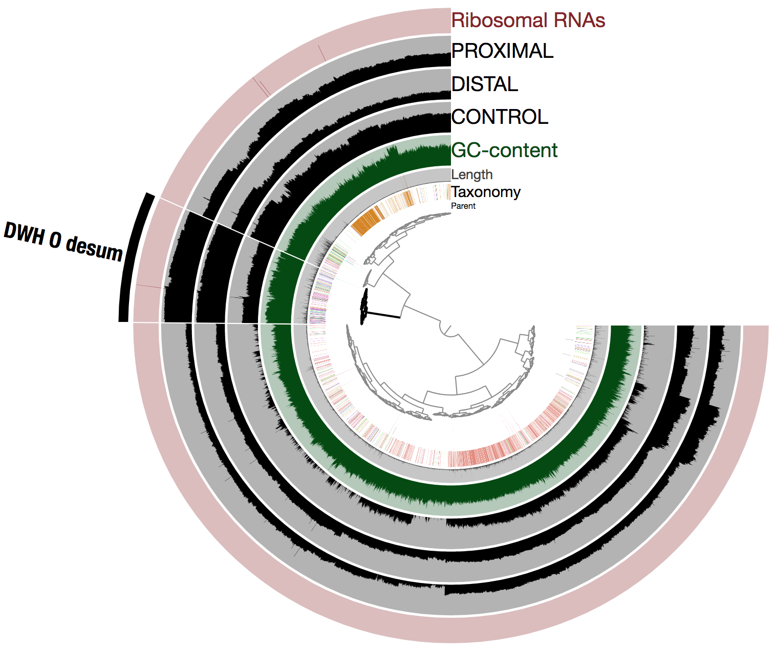
Note that anvi’o produced the tree at the center using both sequence composition and differential coverage. In addition to the taxonomy (determined using Centrifuge) and GC-content, three layers display the mean coverage (in log10) of each scaffold across the metagenomes. The selected cluster contains 526 scaffolds (note that all 6,123 scaffolds are displayed in the figure) and corresponds to DWH O. Desum. Let’s call it DWH O. Desum v2 to avoid any confusion here.

Importantly, DWH O. Desum v2 exhibited dramatic improvements compared to DWH O. Desum v1. As said earlier for the impatients, it is a 2.81 Mbp long, 97.1% complete, 0% redundant population genome, and Average Nucleotide Identity (ANI) when compared to the original population genome (i.e., DWH O. Desum v1) is 99.6% over a length of 1.04 Mbp (this represents almost the entire length of DWH O. Desum v1). In other words, we got the same population genome, except this time it is close to completion, providing an extra 1.74 Mbp to explore and learn from.

To better understand the remarkable abundance of DWH O. Desum in the oil plume, here is the same visualization using the raw mean coverage values (i.e., not in log view):

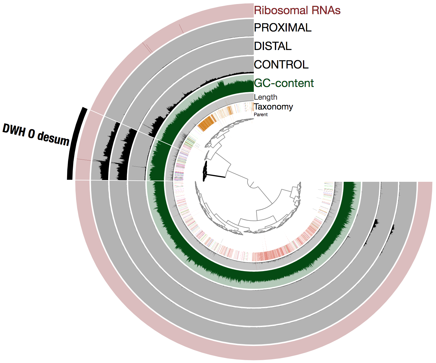
The coverage variations observed between scaffolds of the population genome within each oil plume metagenome (one could intuitively see this as a sign of low quality bin) are likely due to the cumulation of two factors: blooming state leading to a high rate of genomic replications, and the emulsion PCR used to generate the metagenomes. Nevertheless, this did not prevent us from recovering a high quality population genome (with respect to completion) using in part differential coverage across metagenomes to produce the hierarchical tree.

The refining step using only sequence composition

To further support the accuracy of the population genome, we used the anvi-refine program to visualize the 526 scaffolds corresponding to DWH O. Desum v2 using sequence composition only:

anvi-refine -p MERGED/PROFILE.db \
            -c CONTIGS.db \
            -C default \
            -b DWH_O_desum

And here is the display:

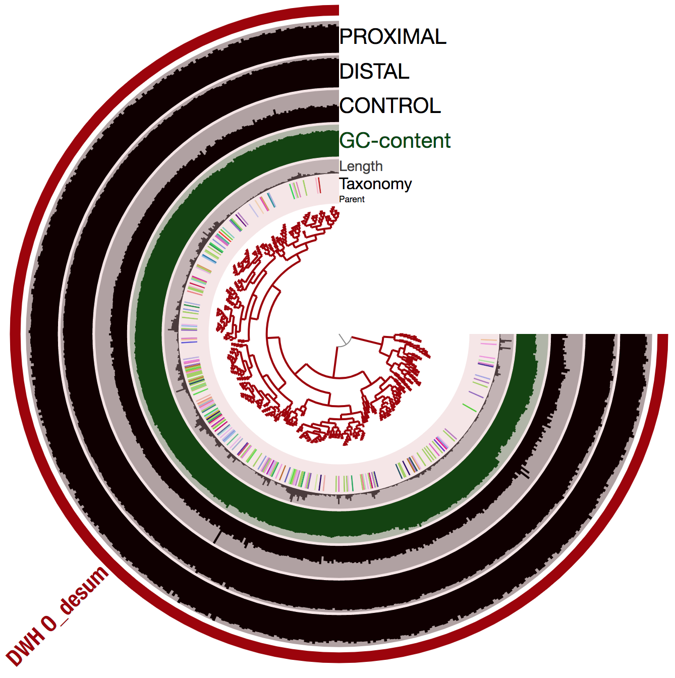
The shape of the inner tree suggests that all scaffolds have a relatively similar tetra nucleotide frequency. This and the coverage trends favor the biological relevance of DWH O. Desum v2. Note that the inconstant taxonomical signal is very common and merely indicates that the genome has not close relative genomes in the reference databases used by Centrifuge.

Here are some statistics about this remarkable population genome:

• Mean coverage: DWH O. Desum v2 mean coverage was 30.2X in the CONTROL metagenome and between 2,579X (PROXIMAL) and 3,529X (DISTAL) in the oil plume metagenomes.

• Relative proportion: DWH O. Desum v2 relative proportion was 0.57% in the CONTROL metagenome (i.e., it recruited 0.57% of the total number of reads) and between 50.7% (PROXIMAL) and 65.7% (DISTAL) in the oil plume metagenomes. This is as expected a considerable gain compared to what DWH O. Desum v1 recruited.

• Taxonomy: CheckM links DWH O. Desum v2 to the family Oceanospirillaceae but cannot resolve its taxonomy at the genus level.

• Similarity to DWH O. desum v1: The Average Nucleotide Identity (ANI) between DWH O. desum v1 and v2 is 99.6% over a length of 1.04 Mbp, which represents almost the entire length of DWH O. Desum v1.

• Similarity to ‘Ca Bermanella macondoprimitus’: The Average Nucleotide Identity (ANI) between DWH O. Desum v2 and the ‘Ca B. macondoprimitus’ by Hu et al. (2017) is 84.3% over 0.95 Mbp. Thus, these two high-quality population genomes (one from the oil plume, the other from an incubation experiment) are very different and likely belong to different genera within the family Oceanospirillaceae.

• alkB gene for oil degradation: DWH O. Desum v2 does not contain the AlkB gene suggested by Hu et al. (2017) to represent the key oil degrading capability of the oil plume bacterial population. This is likely a critical ecological difference between the oil plume population, and the incubation population. Note that to demonstrate the absence of this gene in DWH O. Desum v2, we BLAST searched alkB gene from Hu et al., (2017) against its genomic content (this was done through the RAST platform). The best hit had an e-value of 0.011, and a bit score of 38.

Here is the Alk gene we used for the BLAST:

>Alk gene from Hu et al., (2017)
CTAAGCCATAGCTTTTTTCATTCCTTCACTTTCCACGTCGTAGTGCACTTTCTCAAATGCAGCCAAACCACTTATTTT
GTTGGCGGCGTTAGCCAAGCTAAGTTCTTCGCGTGTGGCGTATTTTTGATCCCATTCTAACACTTTAGGAATCATTAA
CTTATTCCATAACGGAGGAATGAGCGCTACCACCATAGTACTCAAATATCCTCCCACCATCATGGGCGCGTCTGAAAA
TGGTTTTAATTCGTGGTAAGGCACTTCACCTTGTGCATGGTGGTGTGAATGACGGGTTAAGTTAAACATGGCCCAGGA
ACTGGCGCGCTTGTTGGTATTCCATGAATGACGCGGTTGCACTGGTGTTTGTGGATTCCGCACAATGCCATAGTGTTC
CATAAAGTTAACGATTTCCAAGGTGGCTTTACCCCACAGCATGGCCGACACAAAAAATAATGTCCCCGCCCAACCTGC
CATTAGAAAAGCGGCTACCACTAATACTGCGCTCATTAAATAACCTCGTAGGGCCACGTTATGAACGGATAATGTAGA
TTGCCCTTTTTTGGCTAGACGGGCCTGTTCAATTTTCCAGGCACTAATATTACCGCGCACGGTAGAAATTAAAATATG
GGCATATACGTTACGGCCCCTAGGTGCCGTGGCAGGGTCATCTTTGGTACTCACATAACGGTGATGGCCATATACATG
CTCGATGGAGAAGTTTGCATCCCCACTATACGACAGTAACCAGCGACCAATAAACATAGAAATTGGGTCCCAGGTTCG
GTGGGTTAATTCATGGCCGGTAATGGTACCAATCACTCCTATGGATAAACCGGTAAAAATAACCAGGATAATATATTG
AATAAAATCGGTATTTTGTTTGGCCAACAAAATGTCATAACCAGTTAGTTCACTCACCATGGCACCATAACCAAATAT
ATCCGTGGGCGCGAAGTGCCAAACACTTACAAAGCAAATCATGGCAAGAATGGGTAGCGCCAGCCACAACAGCCAGGT
GAGCAGCACAGGGTATTTATATTGGGGTTCGCTGGTGTCGTCACCAAAGAGCAAGTCGGCCCCTATGTAGATGGCAAC
CCAGGCGGCAAAGCCCAAAGCAATATAACTTTCACCCAGGCTAATACTTATAATCGCTATGAGCCCCATAATATGGAT
CGATGAGTATTTTAAATAATGAAACAT

Concluding remarks

Seven years after the disaster, we now have access to the near-complete genome for the bacterial population that once dominated the Deepwater Horizon oil plume. We hope this recovery can contribute to a better characterization of the functional potential, and the contribution of this population to the initial stages of the microbial response to the presence of oil in the environment.

You can access to the history of this discussion here: Ca. Bermanella macondoprimitus is not a strain variant of the oil plume.