Chapter III - Reproducing Kiefl et al, 2022
Table of Contents
- Quick Navigation
- Step 1: Creating a fresh directory
- Step 2: Downloading metagenomes and metatranscriptomes
- Step 3: Downloading SAR11 reference genomes
- Step 4: anvi-run-workflow
- Overview
- Preparing relevant files
- (1) Quality-filtering reads
- (2) ORF prediction (contigs database)
- (3) Mapping reads
- Putting it all together
- Step 5: Exporting gene calls
- Step 6: Function annotation
- Step 7: Isolating HIMB83
- Step 8: Genes and samples of interest
- Step 9: Single codon variants
- Step 10: Single amino acid variants
- Step 11: Structure prediction
- AlphaFold
- Downloading structures
- Importing structures
- Importing pLDDT scores
- Visualizing
- Filtering low quality structures
- Step 12: Relative solvent accessibility
- Step 13: Ligand-binding residue prediction
- Downloading resources
- Running InteracDome on HIMB83
- Exploring and visualizing
- Calculating DTL
- DTL for a custom gene-ligand pair
- Step 14: Calculating pN and pS
- Step 15: Codon properties
- Step 16: Breathe
- Aux. Step 1: Pangenome detour
Quick Navigation
- Chapter I: The prologue
- Chapter II: Configure your system
- Chapter III: Build the data ← you are here
- Chapter IV: Analyze the data
- Chapter V: Reproduce every number
Step 1: Creating a fresh directory
The entire workflow takes place in a single directory, a directory you’ll make now.
Open up your terminal and cd to a place in your filesystem that makes sense to you.
Next, make the following directory, and then cd into it:
Command #1
mkdir kiefl_2021
cd kiefl_2021
‣ Time: Minimal
‣ Storage: Minimal
This is a place you will now call home.
Unless otherwise stated, every command in this workflow assumes you are in this directory. If you’re ever concerned whether you’re in the right place, just type
pwd
The output should look something like: /some/path/that/ends/in/kiefl_2021.
Now that the directory exists, the first thing you’ll populate it with is all of the scripts used in this reproducible workflow. Download them with
Command #2
wget -O ZZ_SCRIPTS.zip https://figshare.com/ndownloader/files/35134069
unzip ZZ_SCRIPTS.zip
rm ZZ_SCRIPTS.zip
‣ Time: Minimal
‣ Storage: Minimal
‣ Internet: Yes
This downloads all of the scripts and puts them in a folder called ZZ_SCRIPTS. If you’re curious, go ahead and look at some or all of them, but don’t get overwhelmed. Each script will be properly introduced when it becomes relevant to the workflow.
Finally, there are some convenience files that will be used, that can be downloaded like so:
Command #3
wget -O TARA_metadata.txt https://figshare.com/ndownloader/files/33108791
wget -O 00_RAW_CORRECT_SIZES https://figshare.com/ndownloader/files/33109079
wget -O 07_SEQUENCE_DEPTH https://figshare.com/ndownloader/files/33953300 # Note to self: Generated via /project2/meren/PROJECTS/KIEFL_2021/ZZ_SCRIPTS/gen_07_SEQUENCE_DEPTH.sh
wget -O config.json https://figshare.com/ndownloader/files/33115685
wget -O SAR11-GENOME-COLLECTION.txt https://figshare.com/ndownloader/files/33117305
‣ Time: Minimal
‣ Storage: Minimal
‣ Internet: Yes
Step 2: Downloading metagenomes and metatranscriptomes
Warning
In this study we rely on metagenomic short reads to access the genetic diversity of naturally occurring SAR11 populations. To a lesser extent, some of our offshoot analyses rely on accompanying metatranscriptomic short reads. As such, this step walks through the process of downloading the collection of metagenomes and metatranscriptomes used in this study.
For those outside the field of metagenomics, the storage requirements of this step may be surprisingly large. 4.1 Tb is definitely nothing to sneeze at, yet unfortunately these files are a necessary evil for anyone who is interested in reproducing the read recruitment experiment, i.e. the alignment of metagenomic and metatranscriptomic reads to the SAR11 reference genomes.
On the brightside, you don’t have to perform this step if you don’t want to. I suspect the majority of people have zero interest in downloading this dataset and subsequently performing the read recruitment experiment. Though the read recruitment is fundamental to our study, reproducing it isn’t very fun or exciting.
For people who fall into this camp, your next stop should be Step 5, where you can download the checkpoint datapack, which contains anvi’o databases that succinctly summarize the results of the read recruitment.
If you want to download the metagenomes/metatranscriptomes, or just want to peruse what I did, read on.
Obtaining the FASTQ metadata
The dataset we used comes from the Tara Oceans Project, which publicly made available a large collection of ocean metagenomes in their Sunagawa et al, 2015 paper, and made available a sister set of ocean metatranscriptomes in their more recent Salazar et al, 2019 paper.
To remain consistent with what we’ve done previously, we used the same 93 metagenomes used in a previous study of ours (here), which corresponds to samples from either the surface (<5 meter depth) or the deep chlorophyll maximum (15-200 meter depth), and that were filtered by a prokaryotic-enriched filter size. Note that these samples exclude the Arctic ocean metagenomes introduced in Salazar et al, 2019. Of these 93 metagenomes, 65 had corresponding metatranscriptomes, which we used in the study.
To download the paired-end FASTQ files of the metagenomes/metatranscriptomes, you have a bash script at ZZ_SCRIPTS/download_fastq_metadata.sh that first constructs the list of FTP links and SRA accession IDs.
Click below to see a line-by-line of the script’s contents.
Show/Hide Script
#! /usr/bin/env bash

# First, download the supplementary info table from the Salazar et al 2019 paper
# (with our naming conventions added as the column `sample_id`)
wget --no-check-certificate -O 00_SAMPLE_INFO_FULL.txt https://figshare.com/ndownloader/files/33109100

# Run a python script that loads in the table (00_SAMPLE_INFO_FULL.txt), subselects all samples that
# were either (1) part of the Delmont & Kiefl et al, 2019
# (https://elifesciences.org/articles/46497), or (2) correspond to a metatranscriptome of a sample
# part of Delmont & Kiefl et al, 2019. Then, output a table of the sample info (00_SAMPLE_INFO.txt)
# and a list of all the accession ids (00_ACCESSION_IDS). Then, construct ftp download links place
# them in a file called 00_FTP_LINKS
python <<EOF
import pandas as pd
df = pd.read_csv('00_SAMPLE_INFO_FULL.txt', sep='\t')
df = df[~df['sample_id'].isnull()]
df.to_csv('00_SAMPLE_INFO.txt', sep='\t', index=False)

x = []
for entry in df['ENA_Run_ID']:
    for e in entry.split('|'):
        x.append(e)
x = list(set(x))

with open('00_ACCESSION_IDS', 'w') as f:
    f.write('\n'.join(x) + '\n')

ftp_template = 'ftp://ftp.sra.ebi.ac.uk/vol1/fastq/{}{}/{}'

with open('00_FTP_LINKS', 'w') as f:
    for e in x:
        if len(e) == 6+3:
            extra = ''
        elif len(e) == 7+3:
            extra = f'/00{e[-1]}'
        elif len(e) == 8+3:
            extra = f'/0{e[-2:]}'
        else:
            raise ValueError("This should never happen")

        ftp = ftp_template.format(e[:6], extra, e)

        f.write(ftp + f'/{e}_1.fastq.gz' + '\n')
        f.write(ftp + f'/{e}_2.fastq.gz' + '\n')
EOF
In summary, it first downloads the file 00_SAMPLE_INFO_FULL.txt, which is in fact an exact replica of the Supplemental Info Table W1 in Salazar et al, 2019, except that an additional column has been added called sample_id that describes our naming convention of samples. It then creates the files 00_ACCESSION_IDS and 00_FTP_LINKS. 00_ACCESSION_IDS contains a list of accession IDs for all FASTQ files to be downloaded. Similarly, 00_FTP_LINKS provides all of the FTP links for these accession IDs.
Go ahead and run this script (internet connection required):
Command #4
./ZZ_SCRIPTS/download_fastq_metadata.sh
‣ Time: <1 min
‣ Storage: Minimal
‣ Internet: Yes
Once finished, you can peruse the outputs like so. head 00_ACCESSION_IDS reveals a preview of its contents:
ERR3587184
ERR3587116
ERR599059
ERR599075
ERR599170
ERR599176
ERR599107
ERR3587141
ERR599017
ERR3586921
Similarly, head 00_FTP_LINKS reveals a preview of its contents:
ftp://ftp.sra.ebi.ac.uk/vol1/fastq/ERR358/004/ERR3587184/ERR3587184_1.fastq.gz
ftp://ftp.sra.ebi.ac.uk/vol1/fastq/ERR358/004/ERR3587184/ERR3587184_2.fastq.gz
ftp://ftp.sra.ebi.ac.uk/vol1/fastq/ERR358/006/ERR3587116/ERR3587116_1.fastq.gz
ftp://ftp.sra.ebi.ac.uk/vol1/fastq/ERR358/006/ERR3587116/ERR3587116_2.fastq.gz
ftp://ftp.sra.ebi.ac.uk/vol1/fastq/ERR599/ERR599059/ERR599059_1.fastq.gz
ftp://ftp.sra.ebi.ac.uk/vol1/fastq/ERR599/ERR599059/ERR599059_2.fastq.gz
ftp://ftp.sra.ebi.ac.uk/vol1/fastq/ERR599/ERR599075/ERR599075_1.fastq.gz
ftp://ftp.sra.ebi.ac.uk/vol1/fastq/ERR599/ERR599075/ERR599075_2.fastq.gz
ftp://ftp.sra.ebi.ac.uk/vol1/fastq/ERR599/ERR599170/ERR599170_1.fastq.gz
ftp://ftp.sra.ebi.ac.uk/vol1/fastq/ERR599/ERR599170/ERR599170_2.fastq.gz
Downloading the FASTQs
Maybe this isn’t your first time downloading FASTQs. Now that you have accession IDs / FTP links in hand, you might prefer downloading these files your own way, such as with fastq-dump or fasterq-dump. Feel free to do this, but just ensure your directory is structured so that FASTQ files remain gzipped and exist in a subdirectory called 00_RAW.
The script responsible for downloading the FASTQs is called ZZ_SCRIPTS/download_fastqs.sh. It places all of the downloaded FASTQs in the directory 00_RAW (a directory it makes automatically). It’s a relatively smart script, that whenever ran, will check the contents of 00_RAW and see what still needs to be downloaded. If a file has only partially downloaded before failing due to a lost connection or what-have-you, this script can tell by comparing your file sizes to the expected file sizes.
Show/Hide Script
Here is the main script:
#! /usr/bin/env bash

# Make a directory called 00_RAW (if it doesn't exists), which houses all of the downloaded FASTQ files
mkdir -p 00_RAW

# Calculate the size of all FASTQ files currently residing in the directory
cd 00_RAW
fastq_count=`ls -1 *.fastq.gz 2>/dev/null | wc -l`
if [ $fastq_count == 0 ]; then
    # There are no fastq.gz files. Create an empty 00_RAW_SIZES
    echo -n "" > ../00_RAW_SIZES
else
    # There exists some fastq.gz files. Populate 00_RAW_SIZES with their sizes
    du *.fastq.gz > ../00_RAW_SIZES
fi
cd ..

# Run a small script that finds which FASTQ files are missing, and which are the wrong sizes
# (corrupt). Then it writes the FTP links of such files to .00_FTP_LINKS_SCHEDULED_FOR_DOWNLOAD
python ZZ_SCRIPTS/download_fastqs_worker.py

remaining=$(cat .00_FTP_LINKS_SCHEDULED_FOR_DOWNLOAD | wc -l)
echo "There are $remaining FASTQs that need to be downloaded/redownloaded"

zero=0
if [[ $remaining -eq $zero ]]; then
    echo "All files have downloaded successfully! There's nothing left to do!"
    exit;
fi

# Download each FASTQ via the ftp links
cd 00_RAW
cat ../.00_FTP_LINKS_SCHEDULED_FOR_DOWNLOAD | while read ftp; do
    # overwrites incomplete files
    filename=$(basename "$ftp")
    wget -O $filename $ftp
done

cd -
And here is the worker script, ZZ_SCRIPTS/download_fastqs_worker.py, that it uses to determine which files are missing/corrupt:
#! /usr/bin/env python

from pathlib import Path
import pandas as pd

ftp_links = pd.read_csv("00_FTP_LINKS", sep='\t', header=None, names=('ftp',))
your_sizes = pd.read_csv("00_RAW_SIZES", sep='\t', header=None, names=('size', 'filepath'))
try:
    my_sizes = pd.read_csv("00_RAW_CORRECT_SIZES", sep='\t', header=None, names=('size', 'filepath'))
except FileNotFoundError as e:
    raise ValueError("You don't have the file 00_RAW_CORRECT_SIZES. Did you forget the step where you download this?")

files_for_download = []
for filepath in my_sizes['filepath']:
    my_size = my_sizes.loc[my_sizes['filepath']==filepath, 'size'].iloc[0]

    matching_entry = your_sizes.loc[your_sizes['filepath']==filepath, 'size']
    if matching_entry.empty:
        # File doesn't exist
        files_for_download.append(filepath)
        continue

    your_size = matching_entry.iloc[0]
    if my_size != your_size:
        # File exists but is wrong
        files_for_download.append(filepath)

with open('.00_FTP_LINKS_SCHEDULED_FOR_DOWNLOAD', 'w') as f:
    ftp_links_for_download = []
    for filepath in files_for_download:
        srr = filepath.split('.')[0]
        ftp_links_for_SRR = ftp_links.ftp[ftp_links.ftp.str.contains(srr)]
        if ftp_links_for_SRR.empty:
            raise ValueError(f"The file 00_FTP_LINKS is missing FTP links for the SRR: {srr}. "
                             f"This really should not happen. My suggestion would be to run "
                             f"`./ZZ_SCRIPTS/download_fastq_metadata.sh` again and see if that fixes it.")
        for ftp_link in ftp_links_for_SRR:
            f.write(ftp_link + '\n')
Since downloading terabytes of data is going to take some time, you’re likely running on a remote server (hosted by your university or what-have-you). Therefore I would recommend safeguarding against unfortunate connection drops that could terminate your session, thereby interrupting your progress. One good solution for linux-based systems is screen, which you can read about here. The gist of screen is that you could run this script in a session that’s uninterrupted when you exit your ssh connection. Alternatively, you could submit this script as a job, assuming you have the ability to submit jobs with long durations.
When ready, go ahead and run the script:
Command #5
./ZZ_SCRIPTS/download_fastqs.sh
‣ Time: 6 days
‣ Storage: 4.1 Tb
‣ Internet: Yes
When the script finally finishes, there should be a folder 00_RAW, containing all the metagenomic/metatranscriptomic FASTQ reads. For me, this took 6 days to complete. Your mileage may vary.
This is currently a single-threaded script. If you end up parallelizing this script because you’re impatient (bless you), please share the script and I’ll add it here.
Verifying the integrity of your downloads
I mentioned earlier that each time ZZ_SCRIPTS/download_fastqs.sh is ran, it checks the presence/absence of all expected files, as well as their expected file sizes. Therefore, you can easily verify the integrity of your downloads by simply running the script again:
Command #6
./ZZ_SCRIPTS/download_fastqs.sh
‣ Time: Minimal
‣ Storage: Minimal
‣ Internet: Yes
Ideally, you want the following output:
There are 0 FASTQs that need to be downloaded/redownloaded
All files have downloaded successfully! There's nothing left to do!
But if you had a shoddy connection, you ran out of disk space, etc., then you will get a message like this:
There are 58 FASTQs that need to be downloaded/redownloaded
(...)
And the process of downloading them will continue. So in summary, check your internet connection, make sure you haven’t run out of storage space, and repeatedly run ZZ_SCRIPTS/download_fastqs.sh until it says you’re done :)
Step 3: Downloading SAR11 reference genomes
In comparison to the last step, this is painless. And you deserve it.
In this study we used already-sequenced SAR11 genomes as targets of a metagenomic and metatranscriptomic read recruitment experiment. That means we take all the reads from a collection of metagenomes and metatranscriptomes, and attempt to align them to SAR11 genomes. The reads that align provide access to the genetic diversity of naturally occurring populations of SAR11.
As it turns out, one of these genomes ended up recruiting magnitudes more than any of the others: this genome is HIMB83, and the genetic diversity captured in the reads aligning to HIMB83 form the foundation of our sequence analyses.
We therefore need some reference SAR11 genomes. We used a genome collection used in a previous paper, which totals 21 unique SAR11 genomes.
We have hosted this genome collection in FASTA format, which you can download with the following command.
Command #7
# Download
wget -O contigs.fa.tar.gz https://figshare.com/ndownloader/files/33114413
tar -zxvf contigs.fa.tar.gz # decompress
rm contigs.fa.tar.gz # remove compressed version
‣ Time: <1 min
‣ Storage: Minimal
‣ Internet: Yes
The downloaded file is named contigs.fa, and meets the anvi’o definition of a contigs-fasta file.
Step 4: anvi-run-workflow
If you opted not to do Step 2 and Step 3, you don’t have the prerequisite files for this step. That’s okay though. You can still read along, or you can skip straight ahead to Step 5, where you can download the checkpoint datapack that contains all the files generated from this step.
Overview
This step covers the following procedures.
- Quality-filtering raw metagenomic and metatranscriptomic reads using illumina-utils.
- Predicting open reading frames for the contigs of each of the 21 SAR11 genomes using Prodigal.
- Competitively mapping short reads from each metagenome and metatranscriptome onto the 21 SAR11 genomes using bowtie2.
We’ve carried this exact procedure out innumerable times in our lab. In fact, this path is so well traversed that Alon Shaiber, a former PhD student in our lab, created anvi-run-workflow, which automates all of these steps using Snakemake.
Because of the automation capabilities of anvi-run-workflow, all of these steps are achievable using a single-line command. That’s a disproportionate amount of computation tied to a single command, so to ensure I don’t blow over important details, I will be chunking this into several sections.
Preparing relevant files
As I mentioned, anvi-run-workflow will do all of the above. But before it can be ran, it needs to be provided a workflow-config that helps it (1) find the files it needs, (2) determine what it should do, and (3) determine how it should do it.
You already have this file. It’s called config.json, and here are it’s line-by-line contents:
Show/Hide config.json
{
    "output_dirs": {
        "CONTIGS_DIR": "03_CONTIGS",
        "MAPPING_DIR": "04_MAPPING",
        "PROFILE_DIR": "05_ANVIO_PROFILE",
        "MERGE_DIR": "06_MERGED",
        "LOGS_DIR": "00_LOGS"
    },
    "workflow_name": "metagenomics",
    "config_version": "2",
    "samples_txt": "samples.txt",
    "fasta_txt": "fasta.txt",
    "iu_filter_quality_minoche": {
        "run": true,
        "--ignore-deflines": true,
        "--visualize-quality-curves": "",
        "--limit-num-pairs": "",
        "--print-qual-scores": "",
        "--store-read-fate": "",
        "threads": 1
    },
    "gzip_fastqs": {
        "run": true,
        "threads": 1
    },
    "anvi_gen_contigs_database": {
        "--project-name": "{group}",
        "--description": "",
        "--skip-gene-calling": "",
        "--ignore-internal-stop-codons": true,
        "--skip-mindful-splitting": "",
        "--contigs-fasta": "",
        "--split-length": "",
        "--kmer-size": "",
        "--skip-predict-frame": "",
        "--prodigal-translation-table": "",
        "threads": 1
    },
    "references_mode": true,
    "bowtie_build": {
        "additional_params": "",
        "threads": 4
    },
    "anvi_init_bam": {
        "threads": 2
    },
    "bowtie": {
        "additional_params": "--no-unal",
        "threads": 2
    },
    "samtools_view": {
        "additional_params": "-F 4",
        "threads": 2
    },
    "anvi_profile": {
        "threads": 2,
        "--sample-name": "{sample}",
        "--overwrite-output-destinations": true,
        "--report-variability-full": "",
        "--skip-SNV-profiling": "",
        "--profile-SCVs": true,
        "--description": "",
        "--skip-hierarchical-clustering": "",
        "--distance": "",
        "--linkage": "",
        "--min-contig-length": "",
        "--min-mean-coverage": "",
        "--min-coverage-for-variability": "",
        "--cluster-contigs": "",
        "--contigs-of-interest": "",
        "--queue-size": "",
        "--write-buffer-size-per-thread": 2000,
        "--max-contig-length": ""
    },
    "anvi_merge": {
        "--sample-name": "{group}",
        "--overwrite-output-destinations": true,
        "--description": "",
        "--skip-hierarchical-clustering": "",
        "--enforce-hierarchical-clustering": "",
        "--distance": "",
        "--linkage": "",
        "threads": 10
    }
}
You should browse workflow-config, the help docs, for a complete description of the format. For now, the most important thing to note is that besides the workflow-config itself, anvi-run-workflow expects only two input files, and these are specified in the workflow-config: a samples-txt and a fasta-txt.
samples-txt
The samples-txt is a tab-delimited file that lets anvi-run-workflow know where all the FASTQ files are and associates each paired-end read set to a user-defined sample name.
To generate the samples-txt, I created a very small python script.
Show/Hide Script
#! /usr/bin/env python

import pandas as pd
from pathlib import Path

df = pd.read_csv('00_SAMPLE_INFO.txt', sep='\t')

samples = {
    'sample': [],
    'r1': [],
    'r2': [],
}

for sample_name, subset in df.groupby('sample_id'):
    errs = []
    for i, row in subset.iterrows():
        errs.extend(row['ENA_Run_ID'].split('|'))

    r1s = []
    r2s = []
    for err in errs:
        r1_path = Path(f"00_RAW/{err}_1.fastq.gz")
        if not r1_path.exists():
            raise ValueError(f"{r1_path} does not exist")

        r2_path = Path(f"00_RAW/{err}_2.fastq.gz")
        if not r2_path.exists():
            raise ValueError(f"{r2_path} does not exist")

        r1s.append(str(r1_path))
        r2s.append(str(r2_path))

    samples['sample'].append(sample_name)
    samples['r1'].append(','.join(r1s))
    samples['r2'].append(','.join(r2s))

samples = pd.DataFrame(samples)
samples.to_csv('samples.txt', sep='\t', index=False)
Run it with the following command:
Command #8
python ZZ_SCRIPTS/gen_samples_txt.py
‣ Time: Minimal
‣ Storage: Minimal
If you get hit with an error similar to ValueError: 00_RAW/ERR3586728_1.fastq.gz does not exist, I’m sure you can guess what’s happened. Something went wrong during Step 3, leading to that file not existing. Go ahead and run ./ZZ_SCRIPTS/download_fastqs.sh to see if the file can be downloaded.
Assuming things ran without error, this generates the file samples.txt, which looks like this:
sample  r1      r2
ANE_004_05M     00_RAW/ERR598955_1.fastq.gz,00_RAW/ERR599003_1.fastq.gz 00_RAW/ERR598955_2.fastq.gz,00_RAW/ERR599003_2.fastq.gz
ANE_004_40M     00_RAW/ERR598950_1.fastq.gz,00_RAW/ERR599095_1.fastq.gz 00_RAW/ERR598950_2.fastq.gz,00_RAW/ERR599095_2.fastq.gz
ANE_150_05M     00_RAW/ERR599170_1.fastq.gz     00_RAW/ERR599170_2.fastq.gz
ANE_150_05M_MT  00_RAW/ERR3587110_1.fastq.gz,00_RAW/ERR3587182_1.fastq.gz       00_RAW/ERR3587110_2.fastq.gz,00_RAW/ERR3587182_2.fastq.gz
ANE_150_40M     00_RAW/ERR598996_1.fastq.gz     00_RAW/ERR598996_2.fastq.gz
ANE_150_40M_MT  00_RAW/ERR3586983_1.fastq.gz,00_RAW/ERR3587104_1.fastq.gz       00_RAW/ERR3586983_2.fastq.gz,00_RAW/ERR3587104_2.fastq.gz
(...)
The r1 and r2 columns specify relative paths to the forward and reverse sets of FASTQ files, respectively, and the left-most column specifies the sample names.
These sample names follow the convention set forth by two other studies in The Meren Lab (here, and here), which have also made primary use of the TARA oceans metagenomes.
In general, the naming convention goes like this:
<region>_<station>_<depth>[_MT]
<region>denotes the region of the sampling site and can be any of- ANE = Atlantic North East
- ANW = Atlantic North West
- ION = Indian Ocean North
- IOS = Indian Ocean North
- MED = Mediterranean Sea
- PON = Pacific Ocean North
- PSE = Pacific South East
- RED = Read Sea
- SOC = South Ocean
-
<station>denotes the station number from where the sample was taken, i.e. the columnStationin00_SAMPLE_INFO_FULL.txt -
<depth>denotes the depth that the sample was taken from in meters, i.e. the columnDepthin00_SAMPLE_INFO_FULL.txt.
Finally, any transcriptome samples are appended with the suffix _MT.
You may notice that a single sample has several SRA accession IDs. For example, ANE_004_05M has 2 FASTQ paths for each forward and reverse set of reads:
sample  r1      r2
ANE_004_05M     00_RAW/ERR598955_1.fastq.gz,00_RAW/ERR599003_1.fastq.gz 00_RAW/ERR598955_2.fastq.gz,00_RAW/ERR599003_2.fastq.gz
This is because ANE_004_05M was sequenced in several batches.
In total, we’re working with 158 samples.
fasta-txt
Just like how samples-txt informs anvi-run-workflow where all the FASTQ files are, fasta-txt informs anvi-run-workflow where all the SAR11 genomes are. contigs.fa contains all of the SAR11 genomes, so the file simply needs to point to contigs.fa.
This is the kind of thing you would normally just manually create. However, since this is a reproducible workflow, I wrote a simple python script, ZZ_SCRIPTS/gen_fasta_txt.py, that generates fasta.txt for you.
Show/Hide Script
#! /usr/bin/env python

with open('fasta.txt', 'w') as f:
    f.write('name\tpath\nSAR11_clade\tcontigs.fa')
Run it like so:
Command #9
python ZZ_SCRIPTS/gen_fasta_txt.py
‣ Time: Minimal
‣ Storage: Minimal
which produces fasta.txt, a very simple file:
name	path
SAR11_clade	contigs.fa
(1) Quality-filtering reads
To remove poor quality reads, I applied a quality filtering step on all of the FASTQ files in samples.txt using the program illumina-utils.
Thanks to the automation capabilities of anvi-run-workflow, this is accomplished via these two items that are already present in config.json:
    "iu_filter_quality_minoche": {
        "run": true,
        "--ignore-deflines": true,
        "--visualize-quality-curves": "",
        "--limit-num-pairs": "",
        "--print-qual-scores": "",
        "--store-read-fate": "",
        "threads": 1
    },
    "gzip_fastqs": {
        "run": true,
        "threads": 1
    },
iu_filter_quality_minoche is the rule specifying the illumina-utils program iu-filter-quality-minoche, and because "run" is set to true, anvi-run-workflow knows that it should run iu-filter-quality-minoche on each FASTQ in samples.txt.
You already have iu-filter-quality-minoche, and you can double check by typing
iu-filter-quality-minoche -v
To conserve space, I opted to gzip all quality-filtered FASTQs, which is specified by the rule gzip_fastqs. Setting "run" to true ensures that after anvi-run-workflow finishes with quality filtering, all subsequent FASTQ files will be gzipped.
Unfortunately, these quality filtered reads will take up another 3.7 Tb of data. If you want to skip this step, modify config.json so that iu_filter_quality_minoche and gzip_fastqs have "run" set to false. You just saved yourself 3.7 Tb of storage. Yes it is that easy.
(2) ORF prediction (contigs database)
I’ve called this procedure “ORF prediction” but it is really much, much more than that. This procedure is truly about creating an anvi’o contigs-db, a database that stores all critical information regarding the SAR11 genome sequences. This database is important because it is a gateway into the anvi’o ecosystem, and later in this workflow you will run anvi’o programs that query, modify, and store information held in this database.
Open reading frames (ORFs) are one type of data stored in the contigs-db and this information is predicted during the creation of a contigs-db, which is carried out by the program anvi-gen-contigs-database. In config.json, we indicate that we want to generate a contigs-db with the following item:
    "anvi_gen_contigs_database": {
        "--project-name": "{group}",
        "--description": "",
        "--skip-gene-calling": "",
        "--ignore-internal-stop-codons": true,
        "--skip-mindful-splitting": "",
        "--contigs-fasta": "",
        "--split-length": "",
        "--kmer-size": "",
        "--skip-predict-frame": "",
        "--prodigal-translation-table": "",
        "threads": 1
    },
This ensures that anvi-gen-contigs-database will be ran, which with these parameters, will predict ORFs with Prodigal. You already have Prodigal, don’t worry… In fact, from now on I’ll stop telling you you have the programs. You have them.
(3) Mapping reads
This portion of the step deals with aligning/recruiting/mapping short reads in samples.txt to the SAR11 genomes in contigs.fa. From now on, I’ll refer to this procedure as “mapping”.
In this study I carry out a competitive read recruitment strategy. What that means is that when a read is mapped, it is compared against all 21 SAR11 genomes in contigs.fa, and is only placed where it maps best. Since we are interested in the population HIMB83 belongs to, providing alternate genomes helps mitigate reads mapping to HIMB83 that are better suited to other genomes. Operationally, this competitive mapping strategy is ensured by putting all the SAR11 genomes within contigs.fa.
The mapping software I used was bowtie2, and the relevant items in config.json are here:
    "references_mode": true,
    "bowtie_build": {
        "additional_params": "",
        "threads": 4
    },
    "bowtie": {
        "additional_params": "--no-unal",
        "threads": 2
    },
"references_mode": true tells anvi-run-workflow to use pre-existing contig sequences, i.e. the SAR11 genome sequences in contigs.fa. This is opposed to an assembly-based metagenomics workflow in which you would first assemble contigs from the FASTQ files, then map the FASTQs onto the assembled contigs.
Mapping with bowtie2 happens in two steps: bowtie2-build builds an index from contigs.fa, and then bowtie2 is ran on each sample, taking the built index and the FASTQs associated with the sample as input.
If you want to pass additional flags to either bowtie2-build or bowtie2 you can do so by modifying the corresponding "additional_params" parameter. As you can see in config.json, the only additional parameter I add is the flag --no-unal, which stands for, ‘no unaligned reads’. This means any reads that don’t map to the reference contigs will be discarded, rather than stored in the output files. Since mapping rates are very low in metagenomic/metatranscriptomic contexts, due to the short reads deriving from thousands of different species, having this parameter is paramount for reducing output file sizes.
For each sample bowtie2 is ran on, a sam-file file is produced, which contains the precise mapping information of each mapped read. This is a space- and speed-inefficient file format designed for human readability, and can and should be converted to a raw-bam-file, which is a human unreadable, space- and speed-efficient counterpart. This step is carried out by samtools, and anvi-run-workflow learns the parameters with which to run samtools from the "samtools_view" item in config.json:
    "samtools_view": {
        "additional_params": "-F 4",
        "threads": 2
    },
    "anvi_init_bam": {
        "threads": 2
    },
Though --no-unal already ensures there are only mapped reads in the sam-file, -F 4 doubly ensures that only mapped reads should be included in the raw-bam-file.
To make querying and accession of these raw-bam-files more efficient, the next step is to convert them to bam-files by indexing them, again with the program samtools. Anvi’o has a program that carries out this samtools utility called anvi-init-bam, which anvi-run-workflow gets instructions to run via the presence of the "anvi_init_bam" item in config.json.
If you zoned out, the mapping results for each sample are stored in a bam-file. To get this mapping information into a format that is understandable by anvi’o, the program anvi-profile takes a single bam-file as input, summarizes its information, and outputs this summary into a database called a single-profile-db. A single-profile-db contains information about coverage, single nucleotide variants, and single codon variants for a given sample, and anvi-run-workflow is given instructions on how to run anvi-profile via the following item:
    "anvi_profile": {
        "threads": 2,
        "--sample-name": "{sample}",
        "--overwrite-output-destinations": true,
        "--report-variability-full": "",
        "--skip-SNV-profiling": "",
        "--profile-SCVs": true,
        "--description": "",
        "--skip-hierarchical-clustering": "",
        "--distance": "",
        "--linkage": "",
        "--min-contig-length": "",
        "--min-mean-coverage": "",
        "--min-coverage-for-variability": "",
        "--cluster-contigs": "",
        "--contigs-of-interest": "",
        "--queue-size": "",
        "--write-buffer-size-per-thread": 2000,
        "--max-contig-length": ""
    },
It is during anvi-profile that codon allele frequencies are calculated from mapped reads (single codon variants). I’ll talk more in depth about that in Step 9, which is dedicated specifically to the topic of exporting single codon variant data from profile databases.
Since there are 285 samples, that’s 285 single-profile-dbs. That’s kind of a pain to deal with. To remedy this, the last instruction specified in config.json is to merge all of the single-profile-dbs together in order to create a profile-db (not a single-profile-db) containing the information from all samples. This is done with the following item:
    "anvi_merge": {
        "--sample-name": "{group}",
        "--overwrite-output-destinations": true,
        "--description": "",
        "--skip-hierarchical-clustering": "",
        "--enforce-hierarchical-clustering": "",
        "--distance": "",
        "--linkage": "",
        "threads": 10
This ensures that anvi-merge, the program responsible for merging mapping data across samples, is ran.
Putting it all together
I’ve done a lot of talking, and its finally time to run anvi-run-workflow.
Here is the command, in all its glory:
anvi-run-workflow -w metagenomics \
                  -c config.json \
                  --additional-params \
                  --jobs <NUM_JOBS> \
                  --resource nodes=<NUM_CORES> \
                  --latency-wait 100 \
                  --rerun-incomplete
Please read on to properly decide <NUM_JOBS>, <NUM_CORES>, and to get some perhaps unsolicited advice on how to submit a command as a job to your cluster.
Cluster configuration
You’ll have to submit this command as a job to your cluster, and you should define <NUM_JOBS> and <NUM_CORES> accordingly. I’m going to assume you have submitted jobs to your cluster in the past and therefore have a reliable approach for submitting jobs. In brief, if your system administrators opted to use the job scheduler SLURM, you’ll submit an sbatch file and if they opted to use Sun Grid Engine (SGE), you’ll submit a qsub script. Those are the two most common options.
At the Research Computing Center of the University of Chicago, we use SLURM, so I made an sbatch file that looked like this:
#!/bin/bash
#SBATCH --job-name=anvi_run_workflow
#SBATCH --output=anvi_run_workflow.log
#SBATCH --error=anvi_run_workflow.log
#SBATCH --partition=meren
#SBATCH --nodes=1
#SBATCH --ntasks-per-node=20
#SBATCH --time=00:00:00
#SBATCH --mem-per-cpu=10000

anvi-run-workflow -w metagenomics \
                  -c config.json \
                  --additional-params \
                  --jobs 20 \
                  --resource nodes=20 \
                  --latency-wait 100 \
                  --rerun-incomplete
You should set <NUM_JOBS> and <NUM_CORES> to the number of the cores the job is submitted with. In my sbatch file I’ve declared I’ll use 20 cores (with the line #SBATCH --ntasks-per-node=20), and so I replaced <NUM_JOBS> and <NUM_CORES> with 20.
Number of threads
Almost done.
If you’re so inclined, now would be a good time to go into config.json and modify the number of threads allotted for each item. For example, anvi-profile will be ran for each sample, and can benefit in speed when given multiple threads. For this reason, I’ve conservatively set the "threads" parameter in the "anvi_profile" item to 2. However, you could set this to 10 if you’re running this job with a lot of cores.
A couple of rules here: (1) No item should have a "threads" parameter that exceeds the value you chose for <NUM_CORES>. (2) The items that benefit from multiple threads are "bowtie_build", "anvi_init_bam", "bowtie", "samtools_view", and "anvi_profile", therefore increasing the "threads" parameter for other items will only slow you down.
If you don’t want to mess with this step, don’t bother. I have purposefully preset the "threads" parameters in config.json to be very practical and I don’t think you’ll have any troubles with the defaults.
Final checks
Make sure this command runs without error:
ls samples.txt fasta.txt config.json
If you encounter an error, one of those files is missing.
Also, make sure you have all of the required FASTQ files by running ZZ_SCRIPTS/download_fastqs.sh one last time:
./ZZ_SCRIPTS/download_fastqs.sh
It should say:
There are 0 FASTQs that need to be downloaded/redownloaded
All files have downloaded successfully! There's nothing left to do!
And finally, do a dry run to make sure anvi-run-workflow is going to run properly:
anvi-run-workflow -w metagenomics \
        -c config.json \
        --additional-params \
        --jobs 20 \
        --resource nodes=20 \
        --latency-wait 100 \
        --rerun-incomplete \
        --dry
The presence of the flag --dry means that Snakemake will go through the motions of the workflow to make sure things are in order, without doing any real computation. As such, this dry run does not need to be submitted to the cluster.
Fire in the hole
You know what how to submit a cluster job, you’ve decided how many cores to submit the job with and subsequently modified <NUM_JOBS>, and <NUM_CORES>, you optionally modified the "threads" parameter for each item in config.json to suit your needs, and you did your final checks. If this is you, there’s nothing left to do but run the thing.
Once again, here is the sbatch file I used, which I named anvi_run_workflow.sbatch:
#!/bin/bash
#SBATCH --job-name=anvi_run_workflow
#SBATCH --output=anvi_run_workflow.log
#SBATCH --error=anvi_run_workflow.log
#SBATCH --partition=meren
#SBATCH --nodes=1
#SBATCH --ntasks-per-node=20
#SBATCH --time=00:00:00
#SBATCH --mem-per-cpu=10000

anvi-run-workflow -w metagenomics \
                  -c config.json \
                  --additional-params \
                  --jobs 20 \
                  --resource nodes=20 \
                  --latency-wait 100 \
                  --rerun-incomplete
and I ran it like so:
sbatch anvi_run_workflow.sbatch
Of course, this information is specific to me. You’ll have to submit your job your own way. However you decide to do it, here is once again the template for the command:
Command #10
anvi-run-workflow -w metagenomics \
                  -c config.json \
                  --additional-params \
                  --jobs <NUM_JOBS> \
                  --resource nodes=<NUM_CORES> \
                  --latency-wait 100 \
                  --rerun-incomplete
‣ Time: ~(1150/<NUM_CORES) hours
‣ Storage: 3.77 Tb (or a mere 150 Gb if skipping quality-filtering)
‣ Memory: Suggested 20 Gb per core
‣ Cluster: Yes
Checking the output
Check the log to see how your job is doing. When it finishes, the last message in the log should be similar to:
[Wed Nov  3 11:45:04 2021]
Finished job 0.
2002 of 2002 steps (100%) done
Complete log: .../kiefl_2021/.snakemake/log/2021-11-01T141742.408307.snakemake.log
After successfully completing, the following directories should exist:
01_QC: Contains all of the quality-filtered FASTQ files (3.62 Tb)03_CONTIGS: The contigs-db of the 21 SAR11 genomes (41 Mb)04_MAPPING: Contains all of the bam-files (94.2 Gb)05_PROFILE: Contains all of the single-profile-dbs (28.1 Gb)06_MERGED: Contains the merged profile-db (28.1 Gb)
If you concerned about space, and you’re positive anvi-run-workflow ran successfully, you can delete 01_QC and 05_PROFILE.
If you want to visualize the fruits of your labor, open up the interactive interface with anvi-interactive:
anvi-interactive -c 03_CONTIGS/SAR11_clade-contigs.db \
                 -p 06_MERGED/SAR11_clade/PROFILE.db
Step 5: Exporting gene calls
Checkpoint datapack
If you have been summoned here, its because you haven’t completed all the previous steps. That’s alright, you can jump in starting from here, assuming you have completed Step 1.
Simply run the following commands, and it will be as if you completed Steps 2 through 4.
(If you completed Steps 2 through 4, don’t run these commands!)
# Downloads the profile database
wget -O 06_MERGED.zip https://figshare.com/ndownloader/files/35160844
unzip 06_MERGED.zip
rm 06_MERGED.zip

# Downloads the contigs database
wget -O 03_CONTIGS.zip https://figshare.com/ndownloader/files/35160838
unzip 03_CONTIGS.zip
rm 03_CONTIGS.zip
Carry on
This marks the end of the journey for analyses that require a computing cluster. If you’ve followed so far, you can continue to work on your computing cluster, or you should feel free to transfer your files to your local laptop/desktop computer, where all of the remaining analyses can be accomplished. In particular, you will need 03_CONTIGS, 06_MERGED, ZZ_SCRIPTS, TARA_metadata.txt, 07_SEQUENCE_DEPTH, and that’s it. Make sure the directory structure remains in tact.
If you decide to transfer files to your local computer and you want to complete Analysis 2 (which is by no means central to the paper), you will either need to bring 04_MAPPING to your local as well (not recommended), or perform Analysis 2 on your computing cluster.
By whatever means you’ve done it, your project directory should have the following items:
./kiefl_2021
├── 03_CONTIGS/
├── 06_MERGED/
├── ZZ_SCRIPTS/
├── TARA_metadata.txt
├── 07_SEQUENCE_DEPTH
(...)
All of the gene coordinates and sequences have been determined using Prodigal and stored in the contigs-db, 03_CONTIGS/SAR11_clade-contigs.db.
However, for downstream purposes it will be useful to have this gene information in a tabular format. Luckily, anvi-export-gene-calls can export this gene info into a gene-calls-txt file. To generate such a file, which we will name gene_calls.txt, simply run the following:
Command #11
anvi-export-gene-calls -c 03_CONTIGS/SAR11_clade-contigs.db \
                       -o gene_calls.txt \
                       --gene-caller prodigal
‣ Time: Minimal
‣ Storage: Minimal
Great.
Step 6: Function annotation
Next, I annotated the genes in this SAR11 genome collection using Pfam, NCBI COGs, and KEGG KOfam. Without these databases, we would have very little conception about what any of these SAR11 genes do.
Short way
If you want to take a shortcut, download this functions file, which contains all of the functions annotated already:
wget -O functions.txt https://figshare.com/ndownloader/files/35134045
Now import it with anvi-import-functions:
anvi-import-functions -c 03_CONTIGS/SAR11_clade-contigs.db \
                      -i functions.txt
Then skip to the next step. Otherwise, continue on.
Long way
First, you need to setup these databases:
Command #12
anvi-setup-kegg-kofams --kegg-snapshot v2020-12-23
anvi-setup-pfams --pfam-version 33.1
anvi-setup-ncbi-cogs --cog-version COG20
‣ Time: ~25 min
‣ Storage: 18.7 Gb
‣ Internet: Yes
If you are using Docker, you can skip this command :)
Now anvi’o has databases that it can search your SAR11 genes against. To annotate from these different sources, run these programs:
Command #13
anvi-run-pfams -c 03_CONTIGS/SAR11_clade-contigs.db -T <NUM_THREADS>
anvi-run-ncbi-cogs -c 03_CONTIGS/SAR11_clade-contigs.db -T <NUM_THREADS>
anvi-run-kegg-kofams -c 03_CONTIGS/SAR11_clade-contigs.db -T <NUM_THREADS>
‣ Time: ~(260/<NUM_THREADS>) min
‣ Storage: Minimal
These functional annotations now live inside 03_CONTIGS/SAR11_clade-contigs.db. To export these functions into a nice tabular output, use the program anvi-export-functions:
Command #14
anvi-export-functions -c 03_CONTIGS/SAR11_clade-contigs.db \
                      -o functions.txt
‣ Time: Minimal
‣ Storage: Minimal
functions.txt is a functions file, and it will be very useful to quickly lookup the predicted functions of any genes of interest, using any of the above sources.
Step 7: Isolating HIMB83
So far, this workflow has indiscriminately included 21 SAR11 genomes. Their sequences are in contigs.fa, they all took part in the competitive read mapping, and consequently they are all in the the contigs-db in 03_CONTIGS/ and the profile-db in 06_MERGED/.
But as you know, this study is really about one genome in particular, HIMB83. As a reminder, the other genomes have been included merely to recruit reads in the competitive mapping experiment, which mitigates the rate that HIMB83 recruits reads that are better-suited to other related and known SAR11 genomes.
To separate HIMB83 from the others, I used the program anvi-split, which chops up a profile-db and contigs-db into smaller pieces. In our case, each piece should be one of the genomes.
To inform anvi-split how it should chop up 03_CONTIGS/03_CONTIGS/SAR11_clade-contigs.db and 06_MERGED/SAR11_clade/PROFILE.db, you need a collection of splits that specifies which contigs correspond to which genomes.
A collection can be imported into anvi’o by creating a collection-txt. You already downloaded the one used in this study and you can find it your directory under the filename SAR11-GENOME-COLLECTION.txt.
SAR11-GENOME-COLLECTION.txt looks like this:
HIMB058_Contig_0001_split_00001 HIMB058
HIMB058_Contig_0001_split_00002 HIMB058
HIMB058_Contig_0001_split_00003 HIMB058
HIMB058_Contig_0001_split_00004 HIMB058
HIMB058_Contig_0002_split_00001 HIMB058
HIMB058_Contig_0002_split_00002 HIMB058
HIMB058_Contig_0002_split_00003 HIMB058
HIMB058_Contig_0003_split_00001 HIMB058
HIMB058_Contig_0003_split_00002 HIMB058
HIMB058_Contig_0003_split_00003 HIMB058
(...)
This can be imported with anvi-import-collection:
Command #15
anvi-import-collection SAR11-GENOME-COLLECTION.txt \
                       -p 06_MERGED/SAR11_clade/PROFILE.db \
                       -c 03_CONTIGS/SAR11_clade-contigs.db \
                       -C GENOMES
‣ Time: <1 min
‣ Storage: Minimal
A collection called GENOMES now exists in 03_CONTIGS/03_CONTIGS/SAR11_clade-contigs.db and 06_MERGED/SAR11_clade/PROFILE.db, which is perfect because this is the collection that we’ll use to run anvi-split. Here is the command:
Command #16
anvi-split -C GENOMES \
           -c 03_CONTIGS/SAR11_clade-contigs.db \
           -p 06_MERGED/SAR11_clade/PROFILE.db \
           -o 07_SPLIT
‣ Time: ~90 min
‣ Storage: 28.3 Gb
‣ Cluster: Yes
If you’re doing this on your laptop, after this program finishes, and are uninterested in completing Analysis 1, you can delete 06_MERGED, freeing up around 28Gb of memory.
The split databases can be found in the output directory 07_SPLIT/, which has the following directory structure:
./07_SPLIT
├── HIMB058
│   ├── AUXILIARY-DATA.db
│   ├── CONTIGS.db
│   └── PROFILE.db
├── HIMB083
│   ├── AUXILIARY-DATA.db
│   ├── CONTIGS.db
│   └── PROFILE.db
├── HIMB114
│   ├── AUXILIARY-DATA.db
│   ├── CONTIGS.db
│   └── PROFILE.db
(...)
Since this study focuses on HIMB83, I wanted to make the database files in 07_SPLIT/HIMB083 more accessible, so I created symbolic links that are in the main directory:
Command #17
ln -s 07_SPLIT/HIMB083/AUXILIARY-DATA.db AUXILIARY-DATA.db
ln -s 07_SPLIT/HIMB083/CONTIGS.db CONTIGS.db
ln -s 07_SPLIT/HIMB083/PROFILE.db PROFILE.db
‣ Time: Minimal
‣ Storage: Minimal
Now you have fast access to these files in the main directory:
ls AUXILIARY-DATA.db CONTIGS.db PROFILE.db
Step 8: Genes and samples of interest
In our study we investigated single codon variants (SCVs) by using the HIMB83 reference genome to recruit reads from different metagenomes. The collection of reads recruited by HIMB83 represent a subclade we call 1a.3.V, and small differences in these reads form the basis of the SCVs we identify within 1a.3.V.
This means (1) we can’t study SCVs in metagenomes where HIMB83 doesn’t recruit reads, and (2) we can’t study SCVs in genes that do not recruit reads.
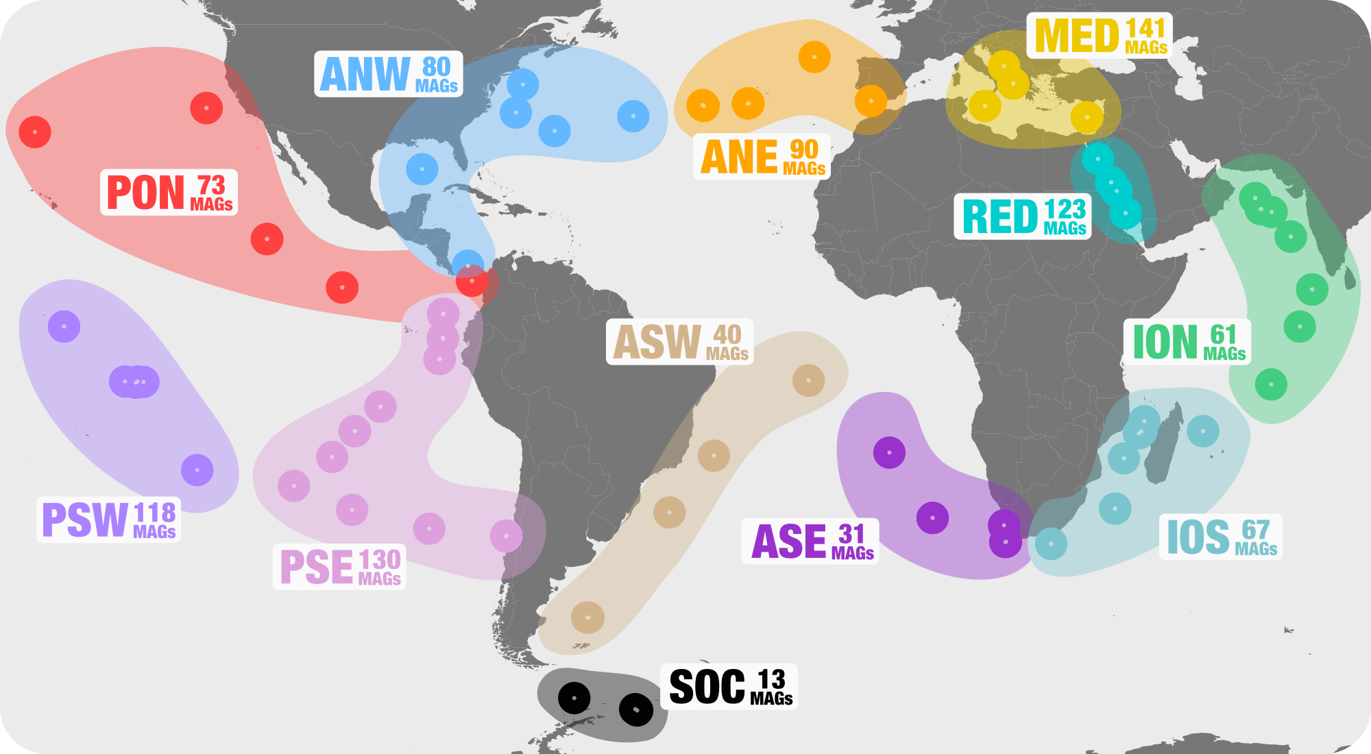
To get what I mean, if you load up the interactive interface you will be greeted with the following view:
anvi-interactive --gene-mode -C DEFAULT -b ALL_SPLITS
Each layer (radius) is a sample (either metagenome or metatranscriptome) and each item (angle) is a gene. The grey-scale color indicates the coverage of a given gene in a given sample. And what we can see is that there are many genes in HIMB83 that are absent in samples (e.g. highlighted in red), and many samples where HIMB83 doesn’t recruit reads (e.g. highlighted in blue).
For all downstream analyses, we get rid of these samples and genes so that we can focus exclusively on (1) samples where 1a.3.V is abundant and (2) genes that are core to 1a.3.V, i.e. present in all samples where 1a.3.V is abundant.
In our previous study we already tackled this very problem. Here is an excerpt from the main text.
(...) To identify core 1a.3.V genes, we used a conservative two-step filtering approach. First, we defined a subset of the 103 metagenomes within the main ecological niche of 1a.3.V using genomic mean coverage values (Supplementary file 1c). Our selection of 74 metagenomes in which the mean coverage of HIMB83 was >50X encompassed three oceans and two seas between −35.2° and +43.7° latitude, and water temperatures at the time of sampling between 14.1°C and 30.5°C (Figure 1—figure supplement 1, Supplementary file 1i). We then defined a subset of HIMB83 genes as the core 1a.3.V genes if they occurred in all 74 metagenomes and their mean coverage in each metagenome remained within a factor of 5 of the mean coverage of all HIMB83 genes in the same metagenome (...)
Despite our displeasure with its oversimplification of a complex problem, and its use of arbitrary cutoffs, we opted to adopt the same filtering strategy in order to create consistency with the previous study.
To recapitulate this, I needed per-sample gene coverage data, so I ran anvi-summarize, a program that snoops around a contigs-db and profile-db in order to calculate exactly this information (and more):
Command #18
anvi-summarize -c CONTIGS.db \
               -p PROFILE.db \
               -C DEFAULT \
               -o 07_SUMMARY \
               --init-gene-coverages
‣ Time: 1 min
‣ Storage: 18 Mb
07_SUMMARY is a summary object that contains a plethora of information. Among the most important, is the per-sample gene coverage data in 07_SUMMARY/bin_by_bin/ALL_SPLITS/ALL_SPLITS-gene_coverages.txt.
I wrote a script called ZZ_SCRIPTS/gen_soi_and_goi.py that takes this per-sample gene coverage data and applies the filter criteria of our last paper.
Show/Hide Script
#! /usr/bin/env python

import pandas as pd
from anvio.terminal import Run

# -----------------------------------------------------------------
# Load in data
# -----------------------------------------------------------------

# Load up the gene coverage data
genes = pd.read_csv("07_SUMMARY/bin_by_bin/ALL_SPLITS/ALL_SPLITS-gene_coverages.txt", sep='\t').set_index("gene_callers_id")

# Load up genome coverage data
genome = pd.read_csv("07_SUMMARY/bins_across_samples/mean_coverage.txt", sep='\t').drop('bins', axis=1)

# Subset metatranscriptomes
metatranscriptomes = genome[[col for col in genome.columns if col.endswith('_MT')]]

# To determine samples and genes of interest, we do not include metatranscriptomes
genome = genome[[col for col in genome.columns if not col.endswith('_MT')]]
genome = genome.T.rename(columns={0:'coverage'})

# -----------------------------------------------------------------
# Determine samples of interest
# -----------------------------------------------------------------

# Filter criteria: mean coverage should be > 50
samples_of_interest = genome.index[genome['coverage'] > 50].tolist()

# Additionally discard samples with coeff. of variation in gene coverages > 1.5
coeff_var = genes[samples_of_interest].std() / genes[samples_of_interest].mean()
samples_of_interest = coeff_var.index[coeff_var <= 1.5].tolist()

# Grab corresponding metatranscriptomes for samples of interest
metatranscriptomes_of_interest = [sample + '_MT' for sample in samples_of_interest if sample + '_MT' in metatranscriptomes]

# -----------------------------------------------------------------
# Determine genes of interest
# -----------------------------------------------------------------

# Establish lower and upper bound thresholds that all gene coverages must fall into
genome = genome[genome.index.isin(samples_of_interest)]
genome['greater_than'] = genome['coverage']/5
genome['less_than'] = genome['coverage']*5

genes = genes[samples_of_interest]

def is_core(row):
    return ((row > genome['greater_than']) & (row < genome['less_than'])).all()

genes_of_interest = genes.index[genes.apply(is_core, axis=1)].tolist()

# -----------------------------------------------------------------
# Summarize the info and write to file
# -----------------------------------------------------------------

run = Run()
run.warning("", header="Sample Info", nl_after=0, lc='green')
run.info('Num metagenomes', len(samples_of_interest))
run.info('Num metatranscriptomes', len(metatranscriptomes_of_interest))
run.info('metagenomes written to', 'soi')

run.warning("", header="Gene Info", nl_after=0, lc='green')
run.info('Num genes', len(genes_of_interest))
run.info('genes written to', 'goi', nl_after=1)

with open('soi', 'w') as f:
    f.write('\n'.join([sample for sample in samples_of_interest]))
    f.write('\n')

with open('goi', 'w') as f:
    f.write('\n'.join([str(gene) for gene in genes_of_interest]))
    f.write('\n')
Run it like so:
Command #19
python ZZ_SCRIPTS/gen_soi_and_goi.py
‣ Time: Minimal
‣ Storage: Minimal
This produces the following output:
Sample Info
===============================================
Num metagenomes ..............................: 74
Num metatranscriptomes .......................: 50
metagenomes written to .......................: soi

Gene Info
===============================================
Num genes ....................................: 799
genes written to .............................: goi
As indicated, we worked with 74 samples, since these are the subset of samples that 1a.3.V was stably present in >50X coverage. Of the 1470 genes in HIMB83, we worked with 799 genes, since it is these genes that maintained coverage values commensurate with the genome-wide average in each of these 74 samples. We consider these the 1a.3.V core genes.
The files produced by this script are soi and goi. soi stands for “samples of interest” and goi stands for “genes of interest”. They are simple lists that look like this:
head goi soi
==> soi <==
ANE_004_05M
ANE_004_40M
ANE_150_05M
ANE_150_40M
ANE_151_05M
ANE_151_80M
ANE_152_05M
ANW_141_05M
ANW_142_05M
ANW_145_05M

==> goi <==
1248
1249
1250
1251
1252
1253
1255
1256
1257
1258
Step 9: Single codon variants
Single codon variants (SCVs) are the meat of our analysis. Taken straight from a draft of this paper, here is our definition:
(...) To quantify genomic variation in 1a.3.V, in each sample we identified codon positions of HIMB83 where aligned metagenomic reads did not match the reference codon. We considered each such position to be a single codon variant (SCV). Analogous to single nucleotide variants (SNVs), which quantify the frequency that each nucleotide allele (A, C, G, T) is observed in the reads aligning to a nucleotide position, SCVs quantify the frequency that each codon allele (AAA, …, TTT) is observed in the reads aligning to a codon position (...)
So in summary, a SCV is defined jointly by (1) a codon position in HIMB83 and (2) the codon allele frequencies found in a given metagenome at that position.
Strategy
The strategy for calculating the codon allele frequency of a given codon in the HIMB83 genome is as follows.
The first step is to identify all reads in a metagenome that align fully to the position. By fully I mean the read should align to all 3 of the nucleotide positions in the codon, with no deletions or insertions. Suppose the number of such reads is $C$–this is considered the coverage of the codon in this metagenome.
Then, by tallying up all of the different codons observed in this 3-nt segment of the $C$ aligned reads, you can say this many were AAA, this many were AAT, this many were AAC, yada, yada, yada. By dividing all these counts by $C$, you end up with the allele frequency of each of the 64 codons at this position in this metagenome, aka the definition of a SCV.
Of course, in this study we calculate millions of SCVs. To be specific, we calculate the codon allele frequencies of each codon position in the 1a.3.V core genes, for each metagenome.
Implementing
So how do you get all this information?
Well, the bam-files in 04_MAPPING/ house the detailed alignment information of each and every mapped read. So the information can be calculated from the bam-files. For example, you could load up a bam-file in a python script and start parsing read alignment info like so:
from anvio.bamops import BAMFileObject, Read
for read in BAMFileObject(f"04_MAPPING/SAR11_clade/ANE_004_05M.bam").fetch('HIMB083_Contig_0001', 17528, 17531):
    print(Read(read))
That simple script yields all of the reads in the sample ANE_004_05M that aligned overtop the 3-nt segment of the HIMB83 genome starting at position 17528:
<anvio.bamops.Read object at 0x12f204588>
 ├── start, end : [17428, 17529)
 ├── cigartuple : [(0, 101)]
 ├── read       : GAGAAATTGAACTTTGCAATTAGAGAAGGTGGAAGAACTGTTGGAGCAGGAGTAGTAACTAAAATTATAGAGTAACTCTATAAATAGGAGTGTAGCTCAAT
 └── reference  : GAAAAATTAAACTTTGCAATCAGAGAAGGTGGAAGAACTGTTGGAGCAGGAGTAGTAACTAAAATTATAGAGTAACTCTATAAATAGGAGTGTAGCTCAAT
<anvio.bamops.Read object at 0x12f204588>
 ├── start, end : [17428, 17529)
 ├── cigartuple : [(0, 101)]
 ├── read       : GAAAAATTAAATTTTGCCATTCGTGAAGGTGGAAGAACTGTTGGAGCAGGAGTAGTAACTAAAATTATAGAGTAACTCTATAAATAGGAGTGTAGCTCAAT
 └── reference  : GAAAAATTAAACTTTGCAATCAGAGAAGGTGGAAGAACTGTTGGAGCAGGAGTAGTAACTAAAATTATAGAGTAACTCTATAAATAGGAGTGTAGCTCAAT
<anvio.bamops.Read object at 0x12f204588>
 ├── start, end : [17429, 17530)
 ├── cigartuple : [(0, 101)]
 ├── read       : AAAAATTAAATTTTGCTATTCGAGAAGGTGGAAGAACTGTTGGAGCAGGAGTAGTAACTAAAATTATAGAGTAACTCTATAAATAGGAGTGTAGCTCAATT
 └── reference  : AAAAATTAAACTTTGCAATCAGAGAAGGTGGAAGAACTGTTGGAGCAGGAGTAGTAACTAAAATTATAGAGTAACTCTATAAATAGGAGTGTAGCTCAATT
<anvio.bamops.Read object at 0x12f204588>
 ├── start, end : [17429, 17531)
 ├── cigartuple : [(0, 72), (1, 1), (0, 8), (2, 2), (0, 20)]
 ├── read       : AGAAGTTAAACTTTGCAATTCGAGAAGGTGGAAGAACTGTTGGTGCTGGAGTAGTAACTAAAATTATAGAGTAAACTCTAT--ATAGGAGTGTAGCTCAATTG
 └── reference  : AAAAATTAAACTTTGCAATCAGAGAAGGTGGAAGAACTGTTGGAGCAGGAGTAGTAACTAAAATTATAGAGT-AACTCTATAAATAGGAGTGTAGCTCAATTG
 (...)
From this info you could start to tally the frequency that each codon aligns to a given codon position.
The bam-files are really the only option to recover codon allele frequencies and this is what is done in our study. However, fortunately, this calculation has already occurred. Indeed, this laborious calculation was carried out during the creation of profile-dbs present in 05_PROFILE. anvi-run-workflow knew to calculate codon allele frequencies because the parameter "--profile-SCVs" was set to true in config.json.
Under the hood
The code responsible for carrying out this calculation lies within the anvi’o codebase and the relevant section can be browsed online (click here).
For whoever is curious, here is a brief summary of what’s going on under the hood. For simplicity I will restrict the procedure to a single gene.
First, an array is initialized with 64 rows (one for each codon) and $L$ columns, where $L$ is the length of the gene, measured in codons.
Then, all reads aligning to the gene are looped through. If a read overhangs the gene’s position, the overhanging segment is trimmed. Then all of the codon positions that the read overlaps with are identified. If the read only partially overlaps with a codon position, that position is excluded. If the read has an indel within the codon position, that position is excluded.
Then, each codon position that the read aligns to is looped through. For each codon position, the codon of the read at that position is noted. For exampe, perhaps the read aligned to position 4 with the codon AAA. Then, the element in the array corresponding to position 4 and codon AAA is incremented by a value of 1. Continuing with the example, position 4 corresponds to column 4 and codon AAA happens to correspond to row 1, so the value at column 4 row 1 is incremented by 1. This is repeated for all aligned codon positions in the read, and then the next read is processed.
By the time all reads have been looped through, the array holds the allele count information for each codon position in the gene. If you divide each column by its sum, you get the allele frequency information for that position.
So where is this information stored? It can be found in a table hidden within PROFILE.db. Each row specifies the codon allele frequencies for each SCV. The column names can be probed like so:
sqlite3 PROFILE.db -header -column ".schema variable_codons"
CREATE TABLE variable_codons (sample_id text, corresponding_gene_call numeric, codon_order_in_gene numeric, reference text, departure_from_reference numeric, coverage numeric, AAA numeric, AAC numeric, AAG numeric, AAT numeric, ACA numeric, ACC numeric, ACG numeric, ACT numeric, AGA numeric, AGC numeric, AGG numeric, AGT numeric, ATA numeric, ATC numeric, ATG numeric, ATT numeric, CAA numeric, CAC numeric, CAG numeric, CAT numeric, CCA numeric, CCC numeric, CCG numeric, CCT numeric, CGA numeric, CGC numeric, CGG numeric, CGT numeric, CTA numeric, CTC numeric, CTG numeric, CTT numeric, GAA numeric, GAC numeric, GAG numeric, GAT numeric, GCA numeric, GCC numeric, GCG numeric, GCT numeric, GGA numeric, GGC numeric, GGG numeric, GGT numeric, GTA numeric, GTC numeric, GTG numeric, GTT numeric, TAA numeric, TAC numeric, TAG numeric, TAT numeric, TCA numeric, TCC numeric, TCG numeric, TCT numeric, TGA numeric, TGC numeric, TGG numeric, TGT numeric, TTA numeric, TTC numeric, TTG numeric, TTT numeric);
sample_id, corresponding_gene_call, codon_order_in_gene uniquely specify which SCV the allele frequencies belong to. reference specifies was the codon in the HIMB83 genome at that position is. And finally AAA, …, TTT all specify how many aligned reads corresponded to each of the 64 codons.
This table is 18,740,639 rows, and contributes the majority of PROFILE.db’s hefty 4.0 Gb file size.
sqlite3 PROFILE.db "select count(*) from variable_codons"
18740639
Exporting
As mentioned, the raw SCV data sits in a table in PROFILE.db. To export this data, and add additional columns of utility, I used the program anvi-gen-variability-profile. In addition to its dedicated help page, there is also a lengthy blog post you can read to find out more information (click).
The ability for anvi-gen-variability-profile to export single codon variants (SCVs) was developed in conjunction with this study, and has been released as open source software so it may be utilized by the broader community.
anvi-gen-variability-profile generates a variability-profile that this study makes extensive use of for nearly every figure in the paper. To create this variability-profile, which will be named 11_SCVs.txt, run the following command:
Command #20
anvi-gen-variability-profile -c CONTIGS.db \
                             -p PROFILE.db \
                             --samples-of-interest soi \
                             --genes-of-interest goi \
                             --engine CDN \
                             --include-site-pnps \
                             --kiefl-mode \
                             -o 11_SCVs.txt
‣ Time: 70 min
‣ Storage: 6.7 Gb
Check out the help pages if you want a detailed explanation of each parameter and flag. But for the purposes of this study, there are a couple things that need to be pointed out:
--engine CDNspecifies that SCVs should be exported (as opposed to SNVs (--engine NT) or SAAVs (--engine AA)).--include-site-pnpsspecifies that $pN^{(site)}$ and $pS^{(site)}$ values should be calculated for each SCV (row) and added as additional columns. This calculates $pN^{(site)}$ and $pS^{(site)}$ using 3 different choices of reference, totaling 6 additional columns. However in this study the “popular consensus” is chosen as the reference, and hence, it is the columnspN_popular_consensusandpS_popular_consensusthat are used in downstream analyses.--kiefl-modeensures that all positions are reported, regardless of whether they contained variation in any sample. It is better to have these and not need them, then to need them and not have them.
Exploring
Because the variability-profile for 1a.3.V is so foundational to this study, I wanted to take a little time to reiterate that this data is at your fingertips to explore.
For example, let’s say you wanted to know the top 10 genes that harbored the least nonsynonymous variation (averaging over samples). A quick way to calculate this would be to average over per-site pN.
Here’s how you could do that in Python:
Show/Hide Script
import pandas as pd

# load up the table
df = pd.read_csv('11_SCVs.txt', sep='\t')

# Grab the 10 genes that had the lowest average rates of per-site nonsynonymous polymorphism
top_10_genes = df.groupby('corresponding_gene_call')\
    ['pN_popular_consensus'].\
    agg('mean').\
    sort_values().\
    iloc[:10].\
    index.\
    tolist()

# Get the Pfam annotations for these 10 genes
functions = pd.read_csv('functions.txt', sep='\t')
functions = functions[functions['gene_callers_id'].isin(top_10_genes)]
functions = functions[functions['source'] == 'Pfam']
functions = functions[['gene_callers_id', 'function', 'e_value']].sort_values('gene_callers_id').reset_index(drop=True)

# Print the results
print(functions)
And here is how you could do that in R:
Show/Hide Script
library(tidyverse)

# Load up the table
df <- read_tsv("11_SCVs.txt")

# Grab the 10 genes that had the lowest average rates of per-site nonsynonymous polymorphism
top_10_genes <- df %>%
    group_by(corresponding_gene_call) %>%
    summarise(mean_pN = mean(pN_popular_consensus, na.rm=T)) %>%
    top_n(-10, mean_pN) %>%
    .$corresponding_gene_call

# Get the Pfam annotations for these 10 genes
functions <- read_tsv("functions.txt") %>%
    filter(
        gene_callers_id %in% top_10_genes,
        `source` == "Pfam",
    ) %>%
    select(gene_callers_id, `function`, e_value) %>%
    arrange(gene_callers_id)

# Print the results
print(functions)
Whichever your preferred language, the result is
   gene_callers_id `function`                                                         e_value
             <dbl> <chr>                                                                <dbl>
 1            1260 Ribosomal protein S10p/S20e                                        6  e-37
 2            1265 Ribosomal protein S19                                              1.5e-37
 3            1552 Bacterial DNA-binding protein                                      1.3e-31
 4            1654 Tripartite ATP-independent periplasmic transporter, DctM component 1.5e-76
 5            1712 'Cold-shock' DNA-binding domain                                    3.2e-26
 6            1712 Ribonuclease B OB domain                                           1.5e- 5
 7            1876 Biopolymer transport protein ExbD/TolR                             7.5e-32
 8            1962 'Cold-shock' DNA-binding domain                                    1.8e-24
 9            1962 Ribonuclease B OB domain                                           1.6e- 5
10            1971 Ribosomal protein L34                                              1.1e-21
11            2003 Ribosomal protein L35                                              2.2e-19
12            2258 Response regulator receiver domain                                 1.8e-23
13            2258 Transcriptional regulatory protein, C terminal                     1.1e-17
We can see that ribosomal proteins dominate the lower spectrum of nonsynonymous polymorphism rates. This is relatively unsurprising, since ribosomal proteins are under strong purifying selection due to the essentiality of protein translation.
I hope this small example has given you some inspiration for how you might explore this data yourself.
Step 10: Single amino acid variants
We also make auxiliary use of single amino acid variants (SAAVs), which are just like SCVs, except the alleles are amino acids instead of codons. This means synonymous codon alleles are pooled together to create each amino acid allele. For more information about the distinction between SCVs and SAAVs, visit this blog post as well as the Methods section.
Exporting
Calculating SAAVs is just as easy as calculating SCVs. The command is mostly the same as Command 20, with the most critical change being the replacement of --engine CDN (codon) to --engine AA (amino acid).
Command #21
anvi-gen-variability-profile -c CONTIGS.db \
                             -p PROFILE.db \
                             --samples-of-interest soi \
                             --genes-of-interest goi \
                             --engine AA \
                             --kiefl-mode \
                             -o 10_SAAVs.txt
‣ Time: 55 min
‣ Storage: 2.9 Gb
Step 11: Structure prediction
AlphaFold
In this section I detail how AlphaFold structures were calculated, and how you can access them. If you’re curious about AlphaFold comparison to MODELLER, check out Analysis 7.
Running AlphaFold is extremely demanding: (1) you need to download terabytes of databases, (2) you realistically need GPUs if doing many predictions, (3) predictions can take several hours per protein, and (4) there doesn’t yet exist (as of November 14, 2021) a proper, non-Dockerized release of the software from Deepmind (see https://github.com/deepmind/alphafold/issues/10).
At the same time, the codebase is evolving rapidly. For example, as of very recently, it now supports protein complex prediction (AlphaFold-Multimer). Concurrently, the community is evolving DeepMind’s project into many different directions, as evidenced by the number of GitHub forks from the official repo recently exceeding 1,100. Some of these projects are gaining more momentum than AlphaFold itself. For example, ColabFold is democratizing the usage of AlphaFold, leveraging Google Colab to remove the entry barriers present in the official project–all while reporting decreased prediction times and increased prediction performance.
My point is that this fast-moving space creates utter chaos for reproducibility. So here’s what I’m going to do.
If you have your own way to run AlphaFold or one of its many variants, feel free to run structure predictions for the HIMB83 genome, in whichever way you want. As a starting point, you’d want a FASTA containing all of HIMB83’s coding proteins, which you can get by running anvi-get-sequences-for-gene-calls:
anvi-get-sequences-for-gene-calls -c CONTIGS.db --get-aa-sequences -o amino_acid_seqs.fa
But for the overwhelming majority, I’m going to provide a download link to a folder containing all the structure predictions. I calculated these using the installation of AlphaFold provided by my system administrator (thank you very much John!). The majority of these structures were ran from this state of the codebase. A single model was used for each prediction using the full_dbs preset, aka the same databases used during the CASP14 competition that brought AlphaFold fame. Using 4-6 GPUs concurrently, these predictions took about a week to complete.
Downloading structures
To save myself a 3.7 Tb upload, and you a 3.7 Tb download, I stripped down the AlphaFold output so that only the structures and their confidence scores remain. Go ahead and download the folder 09_STRUCTURES_AF:
Command #22
wget -O 09_STRUCTURES_AF.tar.gz https://figshare.com/ndownloader/files/33125294
tar -zxvf 09_STRUCTURES_AF.tar.gz
rm 09_STRUCTURES_AF.tar.gz
‣ Time: 1 min
‣ Storage: 570 Mb
Congratulations. You now have, as far as I know, the first structure-resolved proteome of HIMB83, totaling 1466 structure predictions.
The directory of 09_STRUCTURES_AF looks like this:
09_STRUCTURES_AF/
├── pLDDT_gene.txt
├── pLDDT_residue.txt
└── predictions
    ├── 1230.pdb
    ├── 1231.pdb
    ├── 1232.pdb
    ├── 1233.pdb
    ├── 1234.pdb
    ├── 1235.pdb
Each structure prediction is stored in PDB format (extension .pdb) in the subdirectory predictions. The name of the file (e.g. 1232.pdb) corresponds to the gene ID that the prediction is for. In addition, there are two files pLDDT_gene.txt and pLDDT_residue.txt that look this this, respectively:
head 09_STRUCTURES_AF/pLDDT_*
==> 09_STRUCTURES_AF/pLDDT_gene.txt <==
gene_callers_id plddt
2097    92.64866003870453
1668    97.7129432349212
1533    96.36232790789984
2656    88.41058053077586
2521    94.78367308931148
1347    96.85009584629944
2057    94.54371752084121
1394    95.93585073291594
1906    93.71860780834405

==> 09_STRUCTURES_AF/pLDDT_residue.txt <==
gene_callers_id codon_order_in_gene     plddt
2097    0       61.745186221181484
2097    1       66.34906435315496
2097    2       71.22925942767823
2097    3       68.07196628022413
2097    4       74.07983839106177
2097    5       77.62031690262823
2097    6       73.53900145982674
2097    7       77.01163895019288
2097    8       83.27200072516415
pLDDT_residue.txt details how confident AlphaFold is in its prediction of a given residue. This score goes from 0-100, where 100 is very confident and 0 is not. For a qualitative description of how to interpret these scores, see DeepMind’s FAQ. In summary, 90-100 represents high confidence, 70-90 represents decent confidence (overall fold is probably correct), and 0-70 represents low confidence.
On the other hand, pLDDT_gene.txt details a gene’s pLDDT averaged over all it’s residues. It is this score I will be using to filter out low quality predictions.
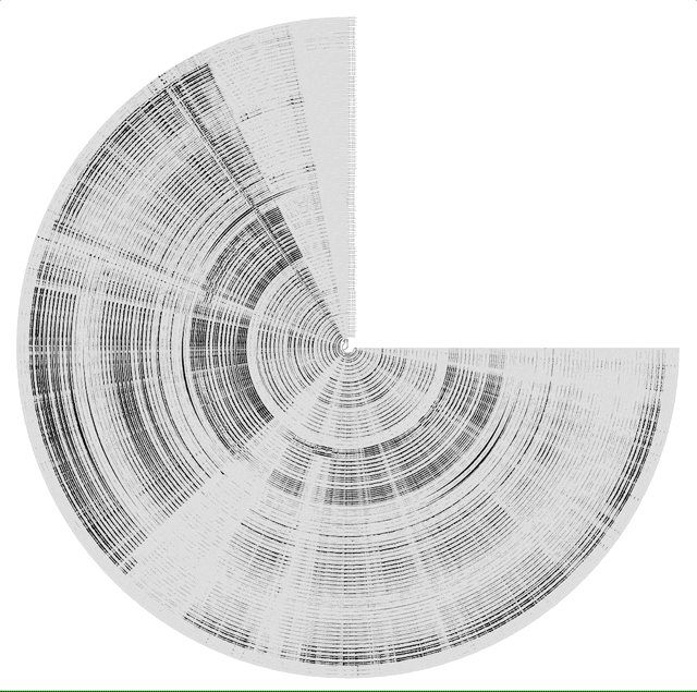
pLDDT at the termini
As a matter of interest, one of the first things I noticed was that pLDDT scores are typically low at the C and N termini. Check out these figures to see what I mean:
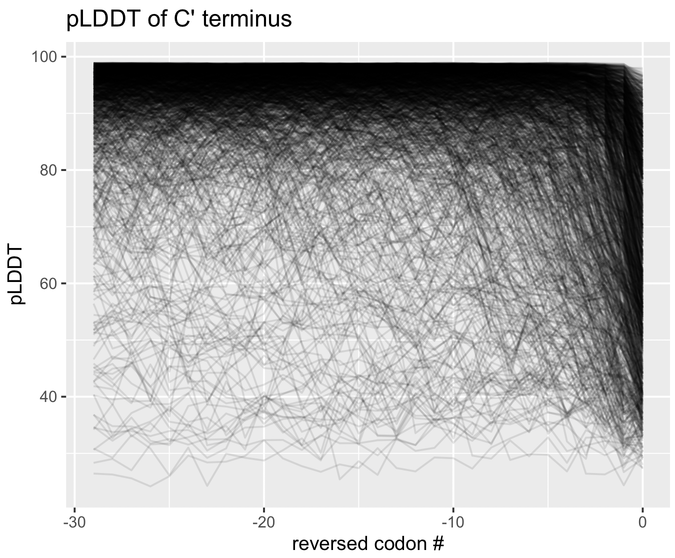
Each line represents the pLDDT scores for one of the 1466 predicted structures. pLDDT scores clearly decay quite dramatically in the first 5-10 residues and the last 5-10 residues. I’m not sure if this is because the telo ends of a protein are intrinsically more disordered, or whether AlphaFold struggles in these regions.
You can generate these figures, too. The script is below.
Show/Hide Script
#! /usr/bin/env Rscript

library(tidyverse)

df <- read_tsv("09_STRUCTURES_AF/pLDDT_residue.txt") %>%
    group_by(gene_callers_id) %>%
    mutate(codon_order_in_gene_rev = codon_order_in_gene - max(codon_order_in_gene))

g <- ggplot(data=df %>% filter(codon_order_in_gene < 30), mapping=aes(codon_order_in_gene, plddt)) +
    geom_line(aes(group=gene_callers_id), alpha=0.1) +
    labs(x='codon #', y='pLDDT', title='pLDDT of N\' terminus')
print(g)

g <- ggplot(data=df %>% filter(codon_order_in_gene_rev > -30), mapping=aes(codon_order_in_gene_rev, plddt)) +
    geom_line(aes(group=gene_callers_id), alpha=0.1) +
    labs(x='reversed codon #', y='pLDDT', title='pLDDT of C\' terminus')
print(g)
Importing structures
To import these structures into a data format understood by anvi’o, you’ll need to create a structure-db. You can do this by providing an external-structures file to the program anvi-gen-structure-database.
There is nothing fancy about an external-structures file–it’s just a 2-column, tab-separated file of gene IDs and the paths to the corresponding protein-structure-txts. I wrote a very tame python script called ZZ_SCRIPTS/gen_external_structures.py that generates the appropriate file.
Show/Hide Script
#! /usr/bin/env python

import pandas as pd
from pathlib import Path

external_structures = {
    'gene_callers_id': [],
    'path': [],
}

structures_dir = Path('09_STRUCTURES_AF/predictions')
for path in structures_dir.glob('*.pdb'):
    gene_id = path.stem
    external_structures['gene_callers_id'].append(gene_id)
    external_structures['path'].append(str(path))

pd.DataFrame(external_structures).to_csv('external_structures.txt', sep='\t', index=False)
Go ahead and run the script like so:
Command #23
python ZZ_SCRIPTS/gen_external_structures.py
‣ Time: Minimal
‣ Storage: Minimal
Here is what the resultant external_structures.txt file looks like:
gene_callers_id	path
1676	09_STRUCTURES_AF/predictions/1676.pdb
2419	09_STRUCTURES_AF/predictions/2419.pdb
1662	09_STRUCTURES_AF/predictions/1662.pdb
2343	09_STRUCTURES_AF/predictions/2343.pdb
1892	09_STRUCTURES_AF/predictions/1892.pdb
2425	09_STRUCTURES_AF/predictions/2425.pdb
2431	09_STRUCTURES_AF/predictions/2431.pdb
1886	09_STRUCTURES_AF/predictions/1886.pdb
2357	09_STRUCTURES_AF/predictions/2357.pdb
(...)
As you can see, its a very basic file. It just says, ‘this gene ID corresponds to this structure’.
Then, to create a structure-db, run anvi-gen-structure-database with the following settings.
Command #24
anvi-gen-structure-database -c CONTIGS.db \
                            --external-structures external_structures.txt \
                            --num-threads <NUM_THREADS> \
                            -o 09_STRUCTURE.db
‣ Time: ~(60/<NUM_THREADS>) min
‣ Storage: 608 Mb
anvi-gen-structure-database was developed in conjunction with this study, and has been released as open source software so it may be utilized by the broader community.
09_STRUCTURE.db is a now a structure-db that holds all of the AlphaFold structures.
Importing pLDDT scores
These proteins can now be readily visualized by anvi’o. But before doing that, I wanted to import the pLDDT scores so they can be visualized too.
Anvi’o has been designed to import various kinds of “miscellaneous data” using the program anvi-import-misc-data, and pLDDT scores fit snugly into this definition of miscellaneous.
Since pLDDT scores exist for each amino acid, this data type is considered to be misc-data-amino-acids, and can be imported into anvi’o by providing a misc-data-amino-acids-txt.
Unfortunately, the format for pLDDT_residue.txt doesn’t quite match the required format for misc-data-amino-acids-txt, but its not far off either. For reasons no one is proud about, anvi’o wants–demands, really–a format that looks like this:
item_name       plddt
2097:0  61.74518622118149
2097:1  66.34906435315496
2097:2  71.22925942767823
2097:3  68.07196628022413
2097:4  74.07983839106177
2097:5  77.62031690262823
(...)
yet pLDDT_residue.txt looks like this:
gene_callers_id codon_order_in_gene     plddt
2097    0       61.745186221181484
2097    1       66.34906435315496
2097    2       71.22925942767823
2097    3       68.07196628022413
2097    4       74.07983839106177
2097    5       77.62031690262823
(...)
This is easily fixed by the script, ZZ_SCRIPTS/gen_plddt_misc_data.py.
Show/Hide Script
#! /usr/bin/env python
import pandas as pd from pathlib import Path
df = pd.read_csv(str(Path(‘09_STRUCTURES_AF/pLDDT_residue.txt’)), sep=’\t’) df[‘item_name’] = df[‘gene_callers_id’].astype(str) + ‘:’ + df[‘codon_order_in_gene’].astype(str) df[[‘item_name’, ‘plddt’]].to_csv(‘plddt_misc_data.txt’, sep=’\t’, index=False)
Run it like so:
Command #25
python ZZ_SCRIPTS/gen_plddt_misc_data.py
‣ Time: Minimal
‣ Storage: 12 Mb
This creates creates a misc-data-amino-acids-txt file called plddt_misc_data.txt, which meets anvi’o’s demands. Finally, import this misc data into the CONTIGS.db with the following:
Command #26
anvi-import-misc-data -c CONTIGS.db \
                      -t amino_acids \
                      plddt_misc_data.txt
‣ Time: Minimal
‣ Storage: 23 Mb
The ability for anvi-import-misc-data to import per-amino acid miscellaneous data was developed in conjunction with this study, and has been released as open source software so it may be utilized by the broader community.
This is great, because the pLDDT scores now exist in CONTIGS.db and can be utilized by other programs, such as anvi-display-structure, which I’ll discuss right now.
Visualizing
At this point, you can open up an interactive interface and begin exploring metagenome-derived sequence variants in the context of AlphaFold-predicted protein structures.
anvi-display-structure -c CONTIGS.db \
                       -p PROFILE.db \
                       -s 09_STRUCTURE.db \
                       --samples-of-interest soi
Though there is no good reason for this, unfortunately anvi-display-structure requires an internet connection. This will be fixed in future (>v7.1) versions of anvi’o.
It is through this interface you can really begin to explore the intersection between structural biology and metagenomics.
For example, here’s Gene #1248, a Serine hydroxymethyltransferase that really doesn’t look ns-polymorphism near its binding site.
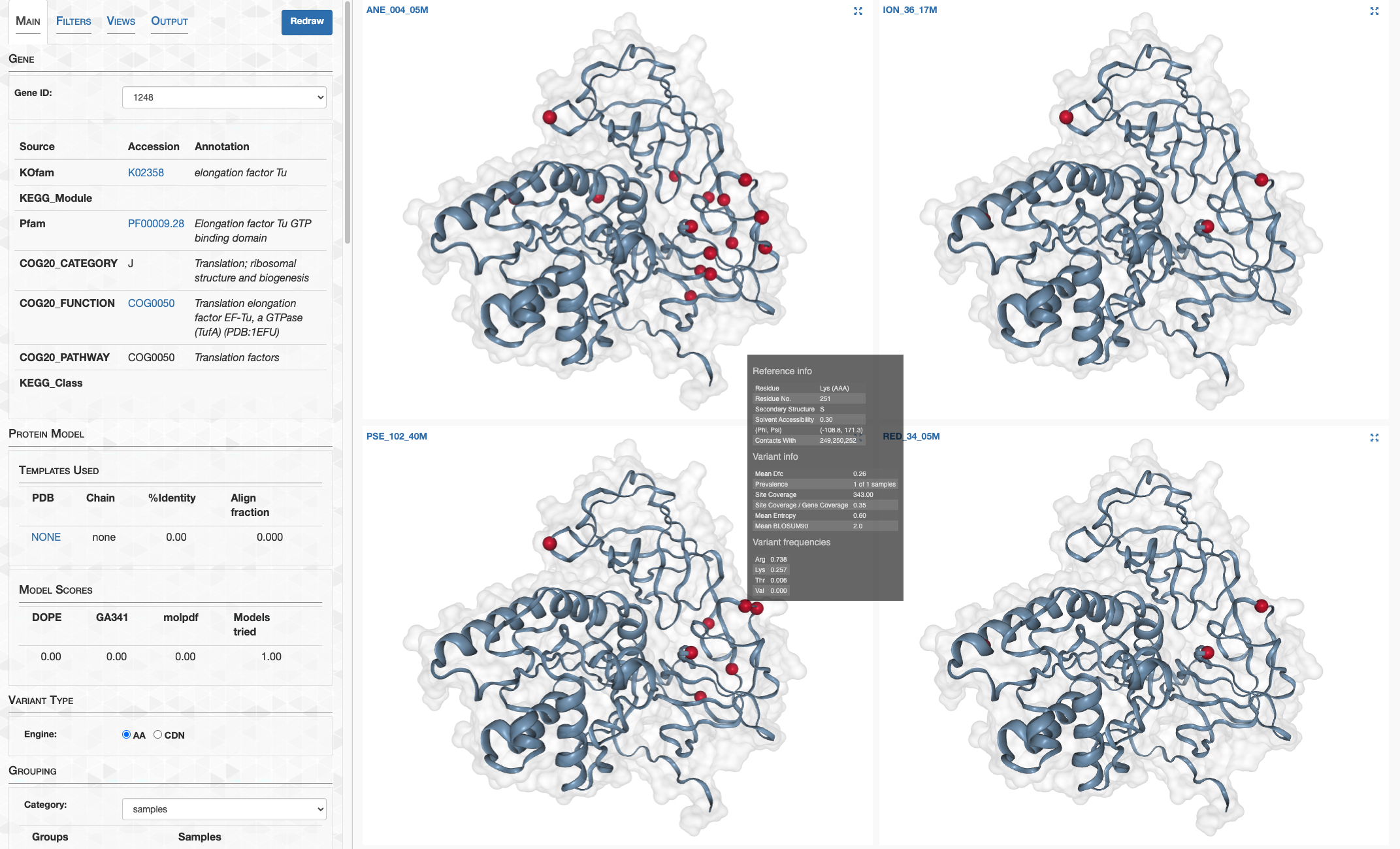
Here’s Gene #2000, a large protein annotated as a phenylalanyl-tRNA synthetase. The surface is colored according to the sample-averaged per-site pN values, where red is high and white is low.
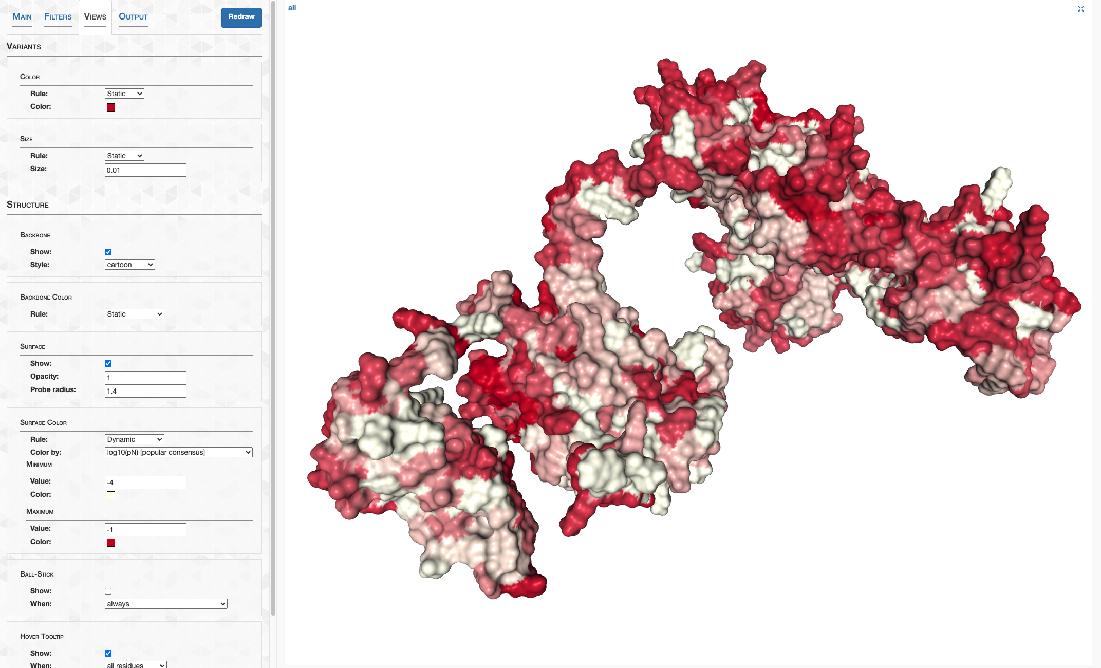
Here is Gene #1298, a putative Holiday junction resolvase. In this instance, I’ve colored the backbone according to the per-site pLDDT score, where red refers to pLDDT < 50, and white refers to pLDDT > 90.
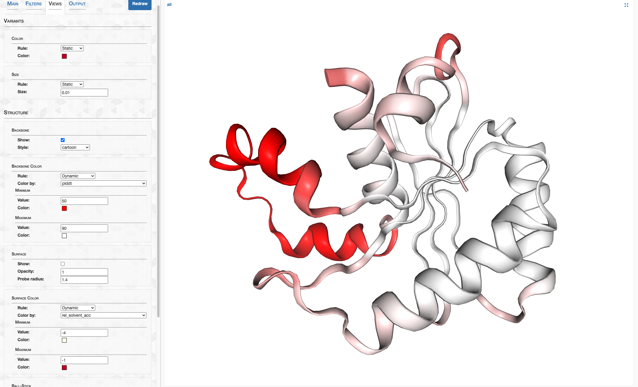
This is obviously a drop in the bucket of what can be explored.
anvi-display-structure was developed in conjunction with this study, and has been released as open source software so it may be utilized by the broader community.
Filtering low quality structures
The last screenshot is a reminder that these are predictions, with some structures yielding low confidence (pLDDT scores) either due to intrinsically disordered regions or poor quality models. Here is a distribution of gene-averaged pLDDT model scores to get an idea of what we’re working with:
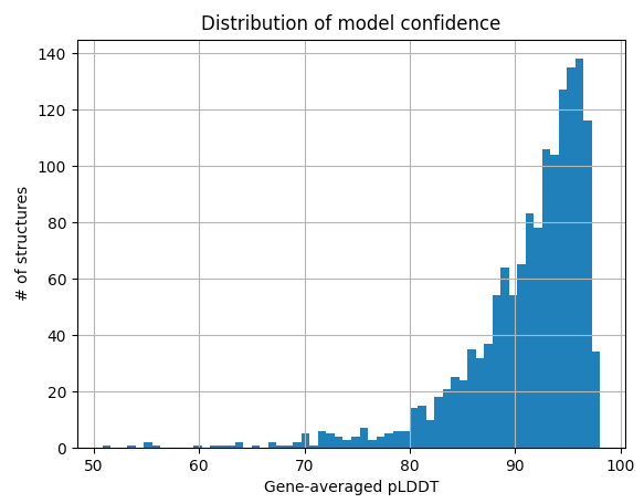
Show/Hide script that made this plot
import pandas as pd
import matplotlib.pyplot as plt
df = pd.read_csv("09_STRUCTURES_AF/pLDDT_gene.txt", sep='\t')
df['plddt'].hist(bins=60)
plt.title('Distribution of model confidence')
plt.xlabel('Gene-averaged pLDDT')
plt.ylabel('# of structures')
plt.show()
Based on AlphaFold’s FAQ, where they qualitatively describe pLDDT, I have conservatively decided to filter out any models with an average pLDDT < 80. To carry out this filtering, I created the script ZZ_SCRIPTS/gen_genes_with_good_structures.py.
Show/Hide gen_genes_with_good_structures.py
#! /usr/bin/env python

import pandas as pd

# Load in the gene-averaged pLDDT scores
df = pd.read_csv("09_STRUCTURES_AF/pLDDT_gene.txt", sep='\t')

# Get the genes of interest (1a.3.V core genes)
goi = [int(gene.strip()) for gene in open('goi').readlines()]

# Filter criteria
min_threshold = df['plddt'] >= 80
is_core = df['gene_callers_id'].isin(goi)
subset = df.loc[min_threshold & is_core, 'gene_callers_id']

# Write to file
subset.to_csv('12_GENES_WITH_GOOD_STRUCTURES', header=False, index=False)
If you want to be more or less conservative, feel free to modify 80 in the script to whatever you please. Then, run it:
Command #27
python ZZ_SCRIPTS/gen_genes_with_good_structures.py
‣ Time: Minimal
‣ Storage: Minimal
This generates a file 12_GENES_WITH_GOOD_STRUCTURES, which contains the gene IDs of 1a.3.V core genes that had predicted structures with an average pLDDT of at least 80. In total, there were 754 of 799 genes considered to have good structures:
wc -l 12_GENES_WITH_GOOD_STRUCTURES
     754 12_GENES_WITH_GOOD_STRUCTURES
Note that the script ZZ_SCRIPTS/gen_genes_with_good_structures.py doesn’t actually filter 09_STRUCTURE.db. All structures, good or bad, remain in the DB. But by using 12_GENES_WITH_GOOD_STRUCTURES, we can subset 09_STRUCTURE.db, 11_SCVs.txt, and any other datasets we may generate, on a whim.
Step 12: Relative solvent accessibility
Description
When anvi-gen-structure-database was ran in the last step, a structure-db I named 09_STRUCTURE.db was created that stores all of the AlphaFold-predicted structures for the HIMB83 genome.
But some very critical per-residue information was also stored, in a table buried away called residue_info. One of the critical data pieces stored in this table is relative solvent accessibility (RSA). If you’ve read the paper, you know how frequently we used this metric.
The residue_info table is calculated by the ever-useful residue annotation software DSSP. Basically, what happens is that DSSP is ran for each protein structure in the external-structures file we passed to anvi-gen-structure-database, and the result is appended to the residue_info table.
To give you an idea of what the means, you can recapitulate this process manually from the command line for a single protein. Here I pick gene #2563:
mkdssp -i 09_STRUCTURES_AF/predictions/2563.pdb -o DSSP_test_2563.txt
If you get mkdssp: command not found, try dssp instead of mkdssp.
This command runs DSSP on gene #2563 and outputs the results to DSSP_test_2563.txt, which looks like this:
cat DSSP_test_2563.txt
==== Secondary Structure Definition by the program DSSP, CMBI version 2.0                          ==== DATE=2021-11-15        .
REFERENCE W. KABSCH AND C.SANDER, BIOPOLYMERS 22 (1983) 2577-2637                                                              .
                                                                                                                               .
COMPND                                                                                                                         .
SOURCE                                                                                                                         .
AUTHOR                                                                                                                         .
   79  1  0  0  0 TOTAL NUMBER OF RESIDUES, NUMBER OF CHAINS, NUMBER OF SS-BRIDGES(TOTAL,INTRACHAIN,INTERCHAIN)                .
  5250.9   ACCESSIBLE SURFACE OF PROTEIN (ANGSTROM**2)                                                                         .
   61 77.2   TOTAL NUMBER OF HYDROGEN BONDS OF TYPE O(I)-->H-N(J)  , SAME NUMBER PER 100 RESIDUES                              .
    0  0.0   TOTAL NUMBER OF HYDROGEN BONDS IN     PARALLEL BRIDGES, SAME NUMBER PER 100 RESIDUES                              .
    2  2.5   TOTAL NUMBER OF HYDROGEN BONDS IN ANTIPARALLEL BRIDGES, SAME NUMBER PER 100 RESIDUES                              .
    0  0.0   TOTAL NUMBER OF HYDROGEN BONDS OF TYPE O(I)-->H-N(I-5), SAME NUMBER PER 100 RESIDUES                              .
    0  0.0   TOTAL NUMBER OF HYDROGEN BONDS OF TYPE O(I)-->H-N(I-4), SAME NUMBER PER 100 RESIDUES                              .
    0  0.0   TOTAL NUMBER OF HYDROGEN BONDS OF TYPE O(I)-->H-N(I-3), SAME NUMBER PER 100 RESIDUES                              .
    0  0.0   TOTAL NUMBER OF HYDROGEN BONDS OF TYPE O(I)-->H-N(I-2), SAME NUMBER PER 100 RESIDUES                              .
    0  0.0   TOTAL NUMBER OF HYDROGEN BONDS OF TYPE O(I)-->H-N(I-1), SAME NUMBER PER 100 RESIDUES                              .
    0  0.0   TOTAL NUMBER OF HYDROGEN BONDS OF TYPE O(I)-->H-N(I+0), SAME NUMBER PER 100 RESIDUES                              .
    0  0.0   TOTAL NUMBER OF HYDROGEN BONDS OF TYPE O(I)-->H-N(I+1), SAME NUMBER PER 100 RESIDUES                              .
    4  5.1   TOTAL NUMBER OF HYDROGEN BONDS OF TYPE O(I)-->H-N(I+2), SAME NUMBER PER 100 RESIDUES                              .
    8 10.1   TOTAL NUMBER OF HYDROGEN BONDS OF TYPE O(I)-->H-N(I+3), SAME NUMBER PER 100 RESIDUES                              .
   41 51.9   TOTAL NUMBER OF HYDROGEN BONDS OF TYPE O(I)-->H-N(I+4), SAME NUMBER PER 100 RESIDUES                              .
    2  2.5   TOTAL NUMBER OF HYDROGEN BONDS OF TYPE O(I)-->H-N(I+5), SAME NUMBER PER 100 RESIDUES                              .
  1  2  3  4  5  6  7  8  9 10 11 12 13 14 15 16 17 18 19 20 21 22 23 24 25 26 27 28 29 30     *** HISTOGRAMS OF ***           .
  0  0  0  1  0  0  0  0  0  0  1  0  0  0  2  0  0  0  0  0  0  0  0  0  0  0  0  0  0  0    RESIDUES PER ALPHA HELIX         .
  0  0  0  0  0  0  0  0  0  0  0  0  0  0  0  0  0  0  0  0  0  0  0  0  0  0  0  0  0  0    PARALLEL BRIDGES PER LADDER      .
  1  0  0  0  0  0  0  0  0  0  0  0  0  0  0  0  0  0  0  0  0  0  0  0  0  0  0  0  0  0    ANTIPARALLEL BRIDGES PER LADDER  .
  0  0  0  0  0  0  0  0  0  0  0  0  0  0  0  0  0  0  0  0  0  0  0  0  0  0  0  0  0  0    LADDERS PER SHEET                .
  #  RESIDUE AA STRUCTURE BP1 BP2  ACC     N-H-->O    O-->H-N    N-H-->O    O-->H-N    TCO  KAPPA ALPHA  PHI   PSI    X-CA   Y-CA   Z-CA            CHAIN
    1    1 A M              0   0  218      0, 0.0     4,-0.1     0, 0.0     0, 0.0   0.000 360.0 360.0 360.0  56.3  -15.0   13.6    4.2
    2    2 A S    >>  +     0   0   61      2,-0.1     4,-1.7     3,-0.1     3,-0.6   0.601 360.0  71.5-126.3 -32.7  -13.5   11.8    1.3
    3    3 A E  H 3> S+     0   0  163      1,-0.2     4,-1.7     2,-0.2     5,-0.1   0.811  96.3  57.3 -59.2 -28.4  -10.4   14.0    0.4
    4    4 A D  H 3> S+     0   0  108      2,-0.2     4,-2.2     3,-0.2    -1,-0.2   0.870 105.3  48.3 -73.0 -36.7   -8.7   12.8    3.6
    5    5 A V  H <> S+     0   0   13     -3,-0.6     4,-3.0     2,-0.2     5,-0.2   0.968 112.2  47.5 -71.1 -49.9   -8.9    9.0    2.7
    6    6 A S  H  X S+     0   0   12     -4,-1.7     4,-2.6     1,-0.2    -2,-0.2   0.914 115.1  47.0 -55.5 -44.6   -7.5    9.5   -0.9
    7    7 A S  H  X S+     0   0   71     -4,-1.7     4,-2.2    -5,-0.2    -1,-0.2   0.919 114.3  45.9 -66.1 -44.3   -4.7   11.6    0.4
    8    8 A K  H  X S+     0   0   83     -4,-2.2     4,-2.6     2,-0.2     5,-0.2   0.922 113.9  48.5 -65.2 -44.5   -3.8    9.2    3.3
    9    9 A V  H  X S+     0   0    0     -4,-3.0     4,-2.5     2,-0.2     5,-0.2   0.966 112.7  48.2 -59.2 -52.4   -3.9    6.1    1.0
   10   10 A K  H  X S+     0   0   48     -4,-2.6     4,-2.7    -5,-0.2    -2,-0.2   0.877 112.8  49.4 -56.4 -41.8   -1.7    7.9   -1.6
   11   11 A K  H  X S+     0   0  112     -4,-2.2     4,-2.9     2,-0.2    -1,-0.2   0.938 111.2  46.6 -63.8 -50.7    0.8    8.9    1.1
   12   12 A I  H  X S+     0   0   23     -4,-2.6     4,-2.7     1,-0.2     5,-0.2   0.912 116.4  47.1 -57.7 -42.2    1.1    5.4    2.7
   13   13 A V  H  X S+     0   0    0     -4,-2.5     4,-2.6    -5,-0.2     6,-0.3   0.911 113.4  46.8 -67.9 -44.6    1.5    3.9   -0.8
(...)
This data is essentially what’s stored in residue_info, except residue_info includes all genes, not just gene #2563. Thanks, DSSP.
Export options
You already have this data in 09_STRUCTURE.db. However, for quick access, you should export the table using anvi-export-table. Here I am opting to use only a subset of the columns that I deemed useful:
Command #28
anvi-export-table 09_STRUCTURE.db \
                  --table residue_info \
                  --fields 'corresponding_gene_call, codon_order_in_gene, sec_struct, rel_solvent_acc, phi, psi' \
                  -o 09_STRUCTURE_residue_info.txt
‣ Time: <1 min
‣ Storage: 17 Mb
This produces 09_STRUCTURE_residue_info.txt, which looks like this:
corresponding_gene_call	codon_order_in_gene	sec_struct	rel_solvent_acc	phi	psi
2419	0	C	0.3125	360.0	146.1
2419	1	E	0.5161290322580645	-131.9	132.2
2419	2	E	0.17258883248730963	-122.9	131.5
2419	3	E	0.4618834080717489	-123.3	138.3
2419	4	E	0.27111111111111114	-113.1	134.4
2419	5	E	0.3983050847457627	-129.1	125.1
(...)
2400	535	E	0.012903225806451613	-132.3	146.7
2400	536	E	0.0	-137.5	136.9
2400	537	E	0.08205128205128205	-127.1	141.8
2400	538	E	0.20304568527918782	-85.7	129.1
2400	539	C	0.27011494252873564	-116.6	360.0
2400	540
sec_struct is a 3-class secondary structure prediction, rel_solvent_acc is RSA, and phi and psi are backbone torsion angles.
You could also access this data programatically using Python. For example, here is a small script that tells us which structure has the largest average RSA.
#! /usr/bin/env python

import anvio.structureops as sops
sdb = sops.StructureDatabase('09_STRUCTURE.db')
res_info = sdb.get_residue_info_for_all()

# Gene with highest average RSA
print(res_info.groupby('corresponding_gene_call')['rel_solvent_acc'].mean().argmax())
print(res_info.groupby('corresponding_gene_call')['rel_solvent_acc'].mean().max())
This outputs the gene ID 1919. With an average RSA of 0.69, there is no way this thing is folded–the majority of its residue’s are completely exposed to water. Indeed, if you load this up in the interactive interface (anvi-display-structure), you can confirm visually that this protein does not fold. If I were to bet, I would say this is an intrinsically disordered protein (IDP). Not the kind of gene you would want to work with in this study. Thankfully, our filtering has done its job because 1919 is absent in our file, 12_GENES_WITH_GOOD_STRUCTURES.
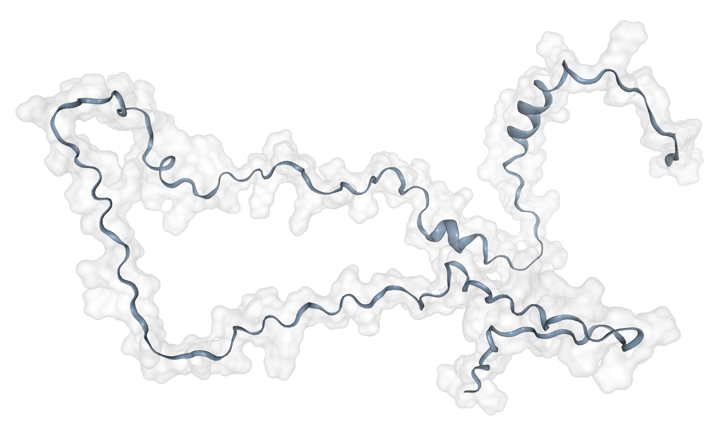
Appending RSA to SCV data
Moving forward, it will prove incredibly useful to add RSA as a column to the variability-profile, 11_SCVs.txt. That way if you become interested in a SCV, you can immediately know its RSA.
To do this, ZZ_SCRIPTS/append_rel_solvent_acc.py appends RSA, as well as the 3-class secondary structure (because why not), to 11_SCVs.txt.
Show/Hide Script
#! /usr/bin/env python

import pandas as pd
import anvio.structureops as sops

# Load the variability table
name = '11_SCVs.txt'
df = pd.read_csv(name, sep='\t')

# Get residue info table from 09_STRUCTURE.db, subset columns to those of interest
sdb = sops.StructureDatabase('09_STRUCTURE.db')
res_info = sdb.get_residue_info_for_all()
columns_of_interest = ['sec_struct', 'rel_solvent_acc']
res_info = res_info[['corresponding_gene_call', 'codon_order_in_gene'] + columns_of_interest]

# Only append residue info if the gene is in 12_GENES_WITH_GOOD_STRUCTURES
goi = [int(x.strip()) for x in open('12_GENES_WITH_GOOD_STRUCTURES').readlines()]
res_info = res_info[res_info['corresponding_gene_call'].isin(goi)]

# Merge the new columns into 11_SCVs.txt, and overwrite
for col in columns_of_interest:
    if col in df.columns:
        df.drop(col, axis=1, inplace=True)
df = df.merge(res_info, how='left', on=['corresponding_gene_call', 'codon_order_in_gene'])

if 'sec_struct' in df.columns:
    # Avoids mixed datatypes
    df['sec_struct'] = df['sec_struct'].astype(str)

df.to_csv(name, sep='\t', index=False)
Make sure you run it:
Command #29
python ZZ_SCRIPTS/append_rel_solvent_acc.py
‣ Time: 26 min
‣ Storage: 300 Mb
Step 13: Ligand-binding residue prediction
In the paper, we predicted how likely certain residues were to be involved in binding to a ligand using the InteracDome database. This resource was introduced by Shilpa Kobren and Mona Singh in their 2018 paper entitled “Systematic domain-based aggregation of protein structures highlights DNA-, RNA- and other ligand-binding positions”.
I’ve written a blog post about InteracDome before, so I’ll borrow a quote that explains the premise:
[One] of the most transformative talks I have ever attended was given by Dr. Mona Singh about her [2018 paper with Shilpa Kobren]. Kobren and Singh took every Pfam family and searched for whether or not any members of the family had crystalized structures that co-complexed with bound ligands. If so, then they calculated 3D distance scores of each residue to the ligand(s) and used these distances as an inverse proxy for binding likelihood (the more likely you are to be involved in the binding of a ligand, the closer you are in physical space to the ligand). They aggregated the totality of these results and ended up with thousands of Pfam IDs for which they could attribute per-residue ligand-binding scores to the Pfam’s associated hidden Markov model (HMM) profile. They used this to extend our knowledge of the human proteome, however when I was listening to the talk all I was thinking about was applying it to metagenomics.
And applying it to metagenomics I did. In fact, that quoted blog post explains in excruciating detail (~4,000 words) exactly how I managed to do that. If you want the details, go read it, or if you want the abridged version, I think it is explained quite well in the Methods section of our study.
Downloading resources
To calculate per-residue ligand-binding scores, the first step is downloading the InteracDome dataset and the Pfam database that it references. This procedure is wrapped up into the simple program anvi-setup-interacdome which creates all of the necessary interacdome-data files.
Command #30
anvi-setup-interacdome
‣ Time: 12 min
‣ Storage: 730 Mb
‣ Internet: Yes
If you are using Docker, you can skip this command :)
Not working? Plan B This step downloads the v31.0 Pfam HMMs using EMBL-EBI’s FTP server. Depending on when you try, your downloads may hang indefinitely. Or they may complete with no problems whatsoever. I have personally experienced both scenarios. Unfortunately, we are really at their mercy when downloading these files. If you try and fail several times, the alternative is to simply download my version of these files:
wget -O Interacdome.tar.gz https://figshare.com/ndownloader/files/33131864
tar -zxvf Interacdome.tar.gz # decompress
rm Interacdome.tar.gz # remove compressed version
This downloads the folder Interacdome. You need to move this folder to a place that anvi’o expects it, which you can do with the following command:
ID_DIR=$(dirname $(which anvi-setup-interacdome))/../anvio/data/misc/
rm -rf $ID_DIR/Interacdome
mv Interacdome/ $ID_DIR
This is the equivalent to having run anvi-setup-interacdome.
anvi-setup-interacdome was developed in conjunction with this study, and has been released as open source software so it may be utilized by the broader community.
Running InteracDome on HIMB83
Once this is ran, you have all of the interacdome-data needed to predict ligand-binding sites on whatever genomes you want.
So how exactly do you do that? To carry out the ligand-binding prediction, I created the program anvi-run-interacdome. Since you didn’t read the blog post I told you to read, here is what anvi-run-interacdome does in 2 sentences, taken straight from the help docs:
In summary, this program runs an HMM search of the genes in your contigs-db to all the Pfam gene families that have been annotated with InteracDome binding frequencies. Then, it parses and filters results, associates binding frequencies of HMM match states to the user’s genes of interest, and then stores the resulting per-residue binding frequencies for each gene into the contigs-db as misc-data-amino-acids.
In the context of this study, here’s what’s going to happen when anvi-run-interacdome is ran. An HMM search is going to be ran that compares the HIMB83 genes against the InteracDome Pfams. Each residue (match state) in each Pfam has been annotated with an estimated ligand-binding ‘score’ ranging from 0 to 1, based on their physical proximity to co-complexed ligands in representative structures of the given Pfam. (Literally speaking, a binding frequency score of $X$ for a given ligand and residue means that of all the structures in the Pfam that contain the ligand, a (Henikoff & Henikoff-weighted) fraction $X$ of them had this residue within 3.6Å of the ligand). After the search is complete, all the matches are processed. For each match, i.e. each instance where a HIMB83 gene matches to a Pfam, the HIMB83 residues are aligned to the profile HMM match states, which allows the per-residue ligand-binding scores from the match states to be directly mapped to the HIMB83 residues.
What a mouthful. Thankfully, running anvi-run-interacdome is easy:
Command #31
anvi-run-interacdome -c CONTIGS.db \
                     --min-binding-frequency 0.5 \
                     -O 08_INTERACDOME \
                     --just-do-it
‣ Time: <1 min
‣ Storage: 50 Mb
I chose to only store ligand binding scores greater than 0.5 (--min-binding-frequency 0.5), which means that for a given residue and ligand, of all the experimental structures in the Pfam containing that ligand, at least 50% of them had the residue (match state) within 3.6Å of the ligand. This filters out residues proximal to ligands in only a minority fraction of experimentally available structures, while retaining residues that were found to be proximal in a majority.
anvi-run-interacdome was developed in conjunction with this study, and has been released as open source software so it may be utilized by the broader community.
Exploring and visualizing
After running this program, some files prefixed with 08_INTERACDOME are created, which are collectively referred to as binding-frequencies-txt data. Feel free to explore that data, however, for this workflow the most the important information, i.e. the per-residue ligand-binding scores, have all been stored in CONTIGS.db as misc-data-amino-acids.
If you want to look at these per-residue ligand-binding scores, you can export the data with anvi-export-misc-data.
anvi-export-misc-data -c CONTIGS.db \
                      -t amino_acids \
                      -D InteracDome \
                      -o binding_freqs.txt
Here is a screenshot after I opened binding_freqs.txt in Excel.
Each column represents a different ligand type. Columns ending in _ refer to classes of molecules defined by Kobren & Singh. For example, LIG_SM_ refers to small molecules. Those that don’t end in _ refer to 3-letter PDB codes that can easily be looked up. For example, in blue I’ve highlighted an entry from the column LIG_DAU. Visiting https://www.rcsb.org/ligand/DAU shows that DAU is 2’deoxy-thymidine-5’-diphospho-alpha-d-glucose. The more you know.
Meanwhile, each row is a residue from the HIMB83 genome, that is specified by the amino_acids column. The format is <gene_callers_id>:<codon_order_in_gene>. For example, the blue-highlighted cell refers to the 133rd codon (counting from 0) in gene #1234. This residue has been given the max ligand-binding score of 1.
Visualizing this data in the context of protein structures could not be easier. Just load up anvi-display-structure:
anvi-display-structure -c CONTIGS.db \
                       -p PROFILE.db \
                       -s 09_STRUCTURE.db \
                       --gene-caller-ids 1234
Notice that we did not provide the filepath to binding_freqs.txt. That data is already stored in CONTIGS.db, and anvi-display-structure knows exactly what to do with it.
Once the interface opens, navigate to Views.

Remove variants by setting Size to 0.01 in Variants
Color the backbone according to the binding frequency to DAU by setting Rule to Dynamic in Backbone Color and selecting LIG_DAU in Color by:
Optionally add a translucent surface colored by LIG_DAU as well, change the colors however you want, and you’ll be presented with the following view:
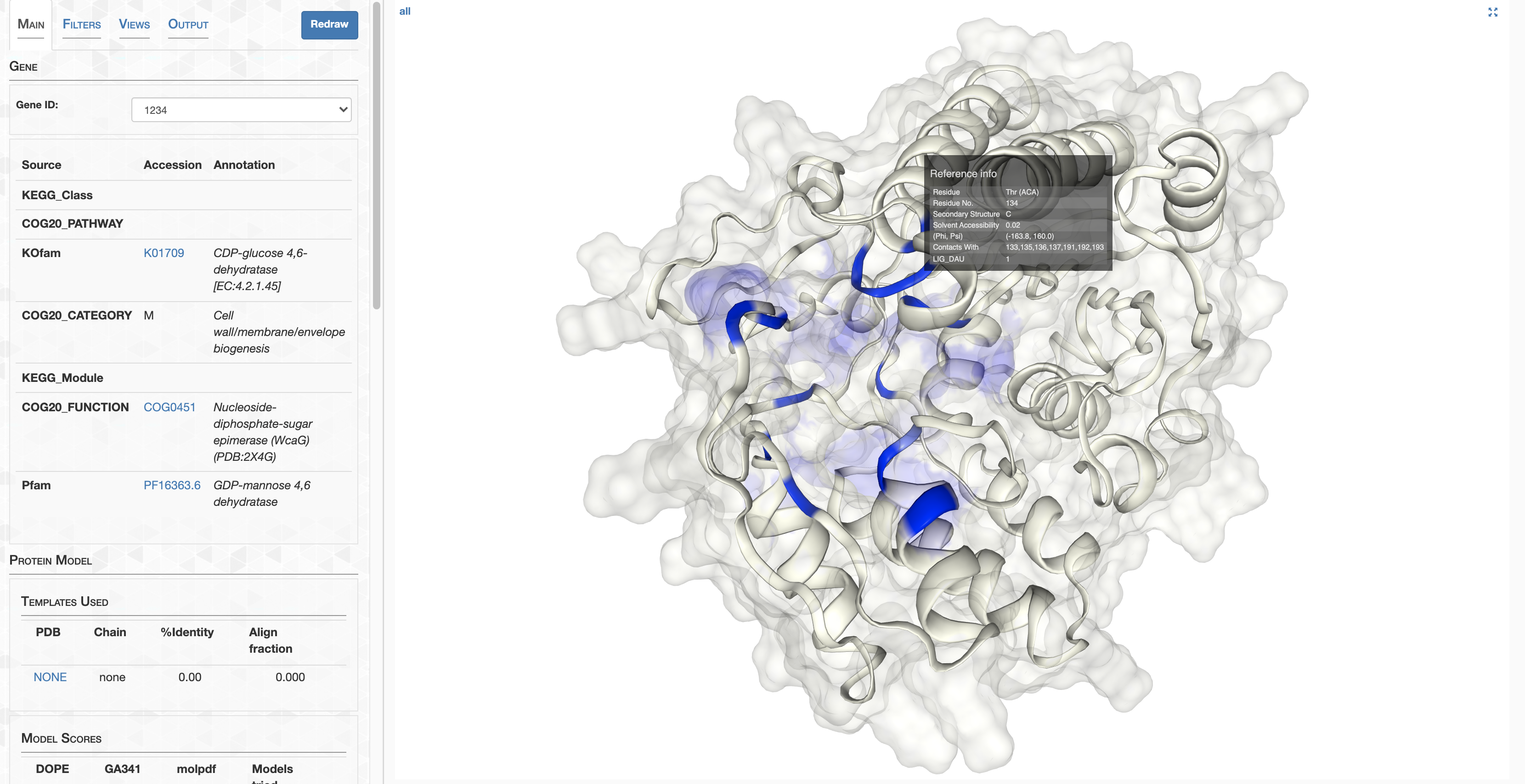
Here, I’m hovering my mouse over the exact residue that is highlighted blue in the Excel sheet. It is satisfying to see that all residues with binding scores > 0.5 congregate in 3D space, even though they occur at different points in the primary sequence.
anvi-display-structure was developed in conjunction with this study, and has been released as open source software so it may be utilized by the broader community.
Calculating DTL
Definition
To define distance-to-ligand (DTL), it’s worth first defining a ligand-binding residue. In the context of this study, I consider a residue in the HIMB83 genome to be a ligand-binding residue if and only if it has a ligand-binding score $\ge 0.5$ for at least one ligand.
How many ligand-binding residues are there?
How many predicted ligand-binding residues are there in HIMB83? To see this we can count the number of lines in the InteracDome table exported with anvi-export-misc-data.
anvi-export-misc-data -c CONTIGS.db \
                      -t amino_acids \
                      -D InteracDome \
                      -o binding_freqs.txt
tail +2 binding_freqs.txt | wc -l # count the lines, excluding header
This yields 11,480 different ligand-binding residues, however this is for all 1472 genes. I wrote a script that subsets this to our 799 genes of interest.
Show/Hide Script
#! /usr/bin/env python

import pandas as pd

# Load up table, create gene ID column
df = pd.read_csv('binding_freqs.txt', sep='\t')
df[['gene_callers_id', 'codon_order_in_gene']] = df['amino_acids'].str.split(':', expand=True)
df['gene_callers_id'] = df['gene_callers_id'].astype(int)

# Load up genes of interest as a list
goi = [g.strip() for g in open('goi').readlines()]

# Filter table by genes of interest
df = df[df['gene_callers_id'].isin(goi)]

# How many ligand-binding residues?
print(df.shape[0])

# How many genes have at least one ligand-binding residue?
print(df['gene_callers_id'].nunique())
The output reveals that 6723 residues are deemed ligand-binding, which is 2.7% of the 251,268 residues in the 1a.3.V core genes. This script also reveals that 521 of 799 genes have at least 1 ligand-binding residue.
Anyways, since InteracDome doesn’t predict the 3D coordinates of ligands, DTL can’t be calculated directly by measuring the Euclidean distance to ligand coordinates. Instead, I defined DTL to be the minimum distance of a residue to any ligand-binding residue. If you assume that residues with estimated binding frequencies $\ge 0.5$ are indeed ligand-binding residues, which of course will not be true in all cases, then this should a pretty decent approximation to the ‘true’ DTL, since ligand-binding residues are by definition in the immediate vicinity of ligands.
One side effect of defining DTL with respect to the closest ligand-binding residue is that by definition, any ligand-binding residue has a DTL of 0.
The last thing to discuss is how distance between residues is measured. We used the Euclidean distance between their side chain center of masses. We also considered a much more primitive distance metric, which was defined not in 3D space but by the distance in sequence. For example, if a gene had only one ligand-binding residue, which occurred at the fifth residue, then the 25th residue would have a DTL of 20. As expected, and as shown in Figure S6, this metric did not perform well.
If you think our methodology for calculating DTL is full of assumptions stacked onto assumptions stacked onto assumptions, we completely agree. To get our full opinion on it, I ask you to please read the following quote from the Results section.
Due to methodological shortcomings, the true predictive power of DTL is undoubtedly higher than we have reported. Errors in structure prediction propagate to errors in DTL, since DTL is calculated using Euclidean distances between residues. Our determination of ligand-binding sites introduces further error for DTL due to incompleteness and uncertainty. For one, binding site predictions exclude (1) ligands that are proteins, (2) ligand-protein complexes that have not co-crystallized with each other, (3) ligands of proteins with no shared homology in the InteracDome database, and (4) unknown ligand-protein complexes. Each of these shortcomings leads to missed binding sites, which leads to erroneously high DTL values in the proximity of unidentified binding sites. Furthermore, our predictions assume that if a homologous protein in the Interacdome database binds to a ligand with a particular residue, then so too does the corresponding residue in the HIMB83 protein. This leads to uncertain predictions, since homology does not necessitate binding site conservancy. Yet despite these methodological shortcomings that one may have expected to shroud biological signals beyond the point of detectability, our methodology remains robust enough for [DTL] to prevail as significant predictors of per-site and per-group variation.
We know its not perfect, but our results show it is still capturing a substantial portion of reality.
Calculating
Because it will prove to be supremely useful, it makes sense to append DTL as a column to the SCVs table, 11_SCVs.txt, such that the DTL for every SCV can be immediately accessed. For this, I created a script, ZZ_SRIPTS/append_dist_to_lig.py.
Show/Hide Script
#! /usr/bin/env python

import numpy as np
import pandas as pd
import argparse
import anvio.dbops as dbops
import anvio.terminal as terminal
import anvio.structureops as sops

from pathlib import Path
from anvio.tables.miscdata import TableForAminoAcidAdditionalData

ap = argparse.ArgumentParser()
ap.add_argument(
    "-A",
    "--all",
    action = "store_true",
    help = "This flag makes --gene, --ligand, and --residues irrelevant. If provided, a column called ANY_dist "
           "is added to every position"
)
ap.add_argument(
    "-g",
    "--gene",
    type = int,
    help = "Which gene are you calculating DTL for?"
)
ap.add_argument(
    "-l",
    "--ligand",
    help = "3-letter code of ligand of interest (don't prepend LIG_)"
)
ap.add_argument(
    "-r",
    "--residues",
    help = "Comma-separated residues to use (codon_order_in_gene). Use instead of --ligand if there is no "
           "predicted ligand, but you have positions where you assume the ligand binds to"
)
ap.add_argument(
    "-f",
    "--frequency-cutoff",
    default = 0.5,
    type = float,
    help = "Residues with ligand-binding scores below this threshold will be ignored. Default is %(default)g"
)
ap.add_argument(
    "-s",
    "--save-as-misc-data",
    action = "store_true",
    help = "This program DTL data to 11_SCVs.txt. But with this flag provided, it will also generate a "
           "misc-data-amino-acids-txt of the DTL values that can be imported into a contigs database "
           "with anvi-import-misc-data."
)
args = ap.parse_args()

run = terminal.Run()
progress = terminal.Progress()

# ----------------------------------------------------------------------------------
# The primary function
# ----------------------------------------------------------------------------------

def get_min_dist_to_lig(structure, lig_positions, var_pos):
    d = {}
    var_res = None

    for lig_pos in lig_positions:
        if structure.pairwise_distances[var_pos, lig_pos] == 0 and var_pos != lig_pos:
            # This distance hasn't been calculated yet. Calculate it
            if var_res is None:
                var_res = structure.get_residue(var_pos)
            lig_res = structure.get_residue(lig_pos)
            structure.pairwise_distances[var_pos, lig_pos] = structure.get_residue_to_residue_distance(var_res, lig_res, 'CA')

        d[lig_pos] = structure.pairwise_distances[var_pos, lig_pos]

    closest = min(d, key = lambda x: d.get(x))
    return closest, d[closest], structure

# ----------------------------------------------------------------------------------
# Getting ligand-binding positions
# ----------------------------------------------------------------------------------

run.warning("", header="Getting ligand-binding positions", lc='green')

if args.all:
    lig_positions_dict = {}
    min_bind_freq = args.frequency_cutoff

    run.info_single('Fetching InteracDome misc-data-amino-acids data')
    # Get the misc-data-amino-acids as a dataframe
    msg = 'Fetched InteracDome misc-data-amino-acids data '
    amino_acid_additional_data = TableForAminoAcidAdditionalData(argparse.Namespace(contigs_db='CONTIGS.db'))
    lig_df = amino_acid_additional_data.get_multigene_dataframe(group_name='InteracDome')

    run.info_single('Filtering InteracDome misc-data-amino-acids data')

    # remove ligand categories
    lig_df = lig_df[[x for x in lig_df.columns if not x.endswith('_')]]
    # filter any row that does not have at least 1 ligand passing the score threshold
    lig_df = lig_df[lig_df[[x for x in lig_df.columns if x not in ('gene_callers_id', 'codon_order_in_gene')]].min(axis=1) >= min_bind_freq]
    # Filter any genes that do not have a good structure
    goi = [int(x.strip()) for x in open('12_GENES_WITH_GOOD_STRUCTURES').readlines()]
    lig_df = lig_df[lig_df['gene_callers_id'].astype(int).isin(goi)]

    for gene_id, group in lig_df.groupby('gene_callers_id'):
        lig_positions_dict[gene_id] = group['codon_order_in_gene'].astype(int).values
else:
    if args.ligand:
        min_bind_freq = args.frequency_cutoff
        amino_acid_additional_data = TableForAminoAcidAdditionalData(argparse.Namespace(contigs_db='CONTIGS.db'))
        lig_df = amino_acid_additional_data.get_gene_dataframe(args.gene, group_name='InteracDome')
        lig_df = lig_df.reset_index(drop=True).set_index('codon_order_in_gene')
        lig_df = lig_df[lig_df['LIG_'+args.ligand].notnull()]
        lig_df = lig_df[lig_df['LIG_'+args.ligand] >= min_bind_freq]
        lig_df = lig_df[['LIG_'+args.ligand]]
        lig_positions = lig_df.index.values
    else:
        # User has chosen to supply residue numbers
        lig_positions = [int(x) for x in args.residues.split(',')]

# ----------------------------------------------------------------------------------
# Calculating DTL for each variant positions
# ----------------------------------------------------------------------------------

#filepath = 'test.txt'
filepath = '11_SCVs.txt'
scvs = pd.read_csv(filepath, sep='\t')
original_order = scvs.index
scvs = scvs.sort_values(by=['corresponding_gene_call', 'codon_order_in_gene'])

sdb = sops.StructureDatabase('09_STRUCTURE.db')

if args.all:
    if args.save_as_misc_data:
        DTLs = {
            'item_name': [],
            'DTL': []
        }
    name = 'ANY'

    scvs[f"{name}_dist"] = np.nan
    scvs[f"{name}_D"] = np.nan

    counter = 0
    progress.new('Adding DTL', progress_total_items=len(lig_positions_dict))

    for gene_id, lig_positions in lig_positions_dict.items():
        progress.increment()
        progress.update(f"{counter+1}/{len(lig_positions_dict)} genes processed")

        structure = sdb.get_structure(gene_id)
        structure_length = len(structure.get_sequence())
        structure.pairwise_distances = np.zeros((structure_length, structure_length))

        scvs_Ds = []
        scvs_dists = []

        scvs_subset = scvs.loc[scvs['corresponding_gene_call'] == gene_id, ['reference', 'codon_order_in_gene']]
        for codon_order_in_gene, scvs_subsubset in scvs_subset.groupby('codon_order_in_gene'):
            reference = scvs_subsubset['reference'].iloc[0]
            size = scvs_subsubset.shape[0]

            if reference in ['TAG', 'TGA', 'TAA']:
                scvs_dists.extend([np.nan]*size)
                scvs_Ds.extend([np.nan]*size)
                continue

            D_closest, d_closest, structure = get_min_dist_to_lig(structure, lig_positions, codon_order_in_gene)
            scvs_dists.extend([d_closest]*size)
            scvs_Ds.extend([abs(D_closest - codon_order_in_gene)]*size)

            if args.save_as_misc_data:
                DTLs['item_name'].append(f"{gene_id}:{codon_order_in_gene}")
                DTLs['DTL'].append(d_closest)

        scvs.loc[scvs['corresponding_gene_call'] == gene_id, f"{name}_dist"] = scvs_dists
        scvs.loc[scvs['corresponding_gene_call'] == gene_id, f"{name}_D"] = scvs_Ds
        counter += 1

else:
    name = args.ligand if args.ligand else 'custom'
    column_name = f"{name}_dist_{args.gene}"
    scvs[column_name] = np.nan

    if args.save_as_misc_data:
        DTLs = {
            'item_name': [],
            column_name: []
        }

    structure = sdb.get_structure(args.gene)
    structure_length = len(structure.get_sequence())
    structure.pairwise_distances = np.zeros((structure_length, structure_length))

    scvs_dists = []

    scvs_subset = scvs.loc[scvs['corresponding_gene_call'] == args.gene, ['reference', 'codon_order_in_gene']]
    for codon_order_in_gene, scvs_subsubset in scvs_subset.groupby('codon_order_in_gene'):
        reference = scvs_subsubset['reference'].iloc[0]
        size = scvs_subsubset.shape[0]
        if reference in ['TAG', 'TGA', 'TAA']:
            scvs_dists.extend([np.nan]*size)
            continue

        D_closest, d_closest, structure = get_min_dist_to_lig(structure, lig_positions, codon_order_in_gene)
        scvs_dists.extend([d_closest]*size)

        if args.save_as_misc_data:
            DTLs['item_name'].append(f"{args.gene}:{codon_order_in_gene}")
            DTLs[column_name].append(d_closest)

    scvs.loc[scvs['corresponding_gene_call'] == args.gene, column_name] = scvs_dists

progress.end()
run.info_single('Now begins the process of saving the new table. This will take some time...', nl_before=1)

# ----------------------------------------------------------------------------------
# Overwrite 11_SCVs with new column
# ----------------------------------------------------------------------------------

if args.all:
    pd.DataFrame(DTLs).to_csv('DTL_misc_data.txt', sep='\t', index=False)
else:
    pd.DataFrame(DTLs).to_csv(f"{column_name}_misc_data.txt", sep='\t', index=False)

scvs.loc[original_order].to_csv(filepath, sep='\t', index=False)
Go ahead and run it:
Command #32
python ZZ_SCRIPTS/append_dist_to_lig.py --all \
                                        --save-as-misc-data
‣ Time: 32 min
‣ Storage: 300 Mb
--alltells the script that DTL should be defined with respect to any ligand-binding residue, no matter the specific type of ligand the residue is predicted to bind to.--save-as-misc-datasays that in addition to appending DTL to11_SCVs.txt, a misc-data-amino-acids-txt file namedDTL_misc_data.txtshould be created so that DTL can be imported intoCONTIGS.db. This is important because it will allow the visualization of DTL while visualizing proteins with anvi-display-structure.
After successfully running this program, DTL is now a column in 11_SCVs.txt named ANY_dist (sorry that the name is cryptic). Additionally, a 1D sequence DTL has also been added as a column named ANY_D.
Additionally, the misc-data-amino-acids-txt file DTL_misc_data.txt has been created that you should import:
Command #33
anvi-import-misc-data -c CONTIGS.db \
                      -t amino_acids \
                      DTL_misc_data.txt
‣ Time: Minimal
‣ Storage: Minimal
While this import may seem inconsequential, this has just opened up a world of exploration. You can now interactively browse this proteome and visualize DTL values with respect to protein structure and sequence variation. Keep reading for a demo.
Exploring
This is a treasure trove of data.
In order to try and convince you of that, moments before writing this very sentence I just opened up the interface like so:
anvi-display-structure -p PROFILE.db \
                       -c CONTIGS.db \
                       -s 09_STRUCTURE.db \
                       --samples-of-interest soi
Then I selected the first 1a.3.V core gene (Gene #1248) found in the genes of interest file, goi, and within 2 minutes created this figure which is biologically interpretable.
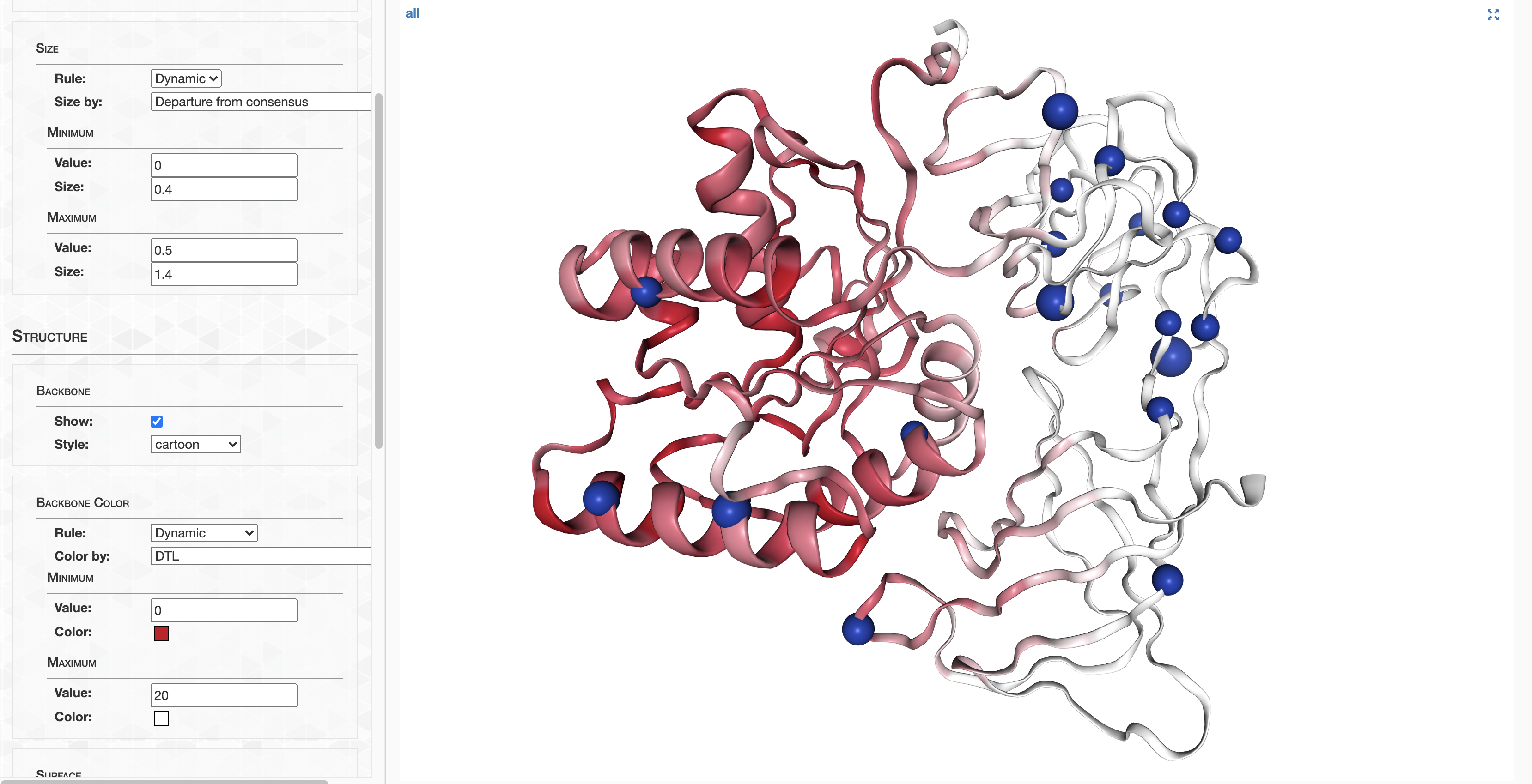
This is the AlphaFold-predicted structure for Gene #1248, a GTPase.
The backbone is colored dynamically according to the residue’s predicted DTL, where low DTL refers to red and high DTL refers to white.
These DTL values were calculated from 11 putative ligands: BEF, CA, FUA, G4P, GCP, GDP, GNP, GSP, GTP, KIR, and MG. Although there is significant diversity in the predicted ligands, all of them are predicted to bind in a relatively conserved region of the protein, as can be seen by the anisotropic DTL values. This means that without consulting an expert on GTPase, we are unable to pinpoint which ligand(s) this protein binds to, but can be relatively certain that such ligand(s) bind in the region indicated in red.
This is reflected in the observed distribution of nonsynonymous variation. In blue spheres are residues in which the sample-averaged amino acid allele frequencies exceeded a departure from consensus >10%. In other words, when pooling across samples, of all the reads that aligned to these positions, >10% of them resolved to amino acids different from the dominant amino acid. The radius of the spheres is proportional to their departure from consensus. Given that we know the binding site is on the left-hand side of the protein, it is therefore of no surprise that the distribution of these positions is heavily favored towards the right-hand side (high DTL) of the protein, since nonsynonymous variation on the left-hand side (low DTL) is far more likely to be purified.
DTL for a custom gene-ligand pair
There are no commands in this section, just some general guidance for if you want to calculate DTL for specific gene-ligand pairs.
When calculating DTL at the scale of hundreds of genes, defining DTL agnostically in terms of the distance to any predicted ligand is the best we can do. This obviously will lead to inaccuracies due to incorrect/missing ligand predictions, although it is clear from the trends in our paper (and even in the example shown with Gene #1248 above) that biology prevails and these inaccuracies do not muddy the signal beyond recognition.
In more targeted instances where you are interested in a single gene, and may have prior knowledge of the binding site, it may make more sense to define DTL with respect to that particular ligand. For example, gene #1326, a Serine hydroxymethyltransferase (SHMT) has a primary binding site where glycine and serine are interconverted.
In this case, since we know a priori what SHMT does, one could define DTL specifically in terms of the distance to predicted serine-binding residues, aka residues with ligand-binding scores >0.5 to the ligand SER.
If you’re curious which residues these are, you can run the following python script:
import argparse
from anvio.tables.miscdata import TableForAminoAcidAdditionalData
amino_acid_additional_data = TableForAminoAcidAdditionalData(argparse.Namespace(contigs_db='CONTIGS.db'))
df = amino_acid_additional_data.get_multigene_dataframe(group_name='InteracDome')
ser_binding_residues = df.loc[
    (df['LIG_SER'].notnull()) & (df['gene_callers_id']==1326),
    ['codon_order_in_gene', 'LIG_SER']
].reset_index(drop=True)
print(ser_binding_residues)
Which yields the responsible residues and their binding scores:
data_key  codon_order_in_gene   LIG_SER
0                          46  1.000000
1                         137  0.799588
2                         215  0.799588
3                         241  0.516195
4                         373  1.000000
You can open up the interactive interface and visualize the location of these 5 residues by coloring the backbone color dynamically by the variable LIG_SER:
anvi-display-structure -p PROFILE.db \
                       -c CONTIGS.db \
                       -s 09_STRUCTURE.db \
                       --gene-caller-ids 1326
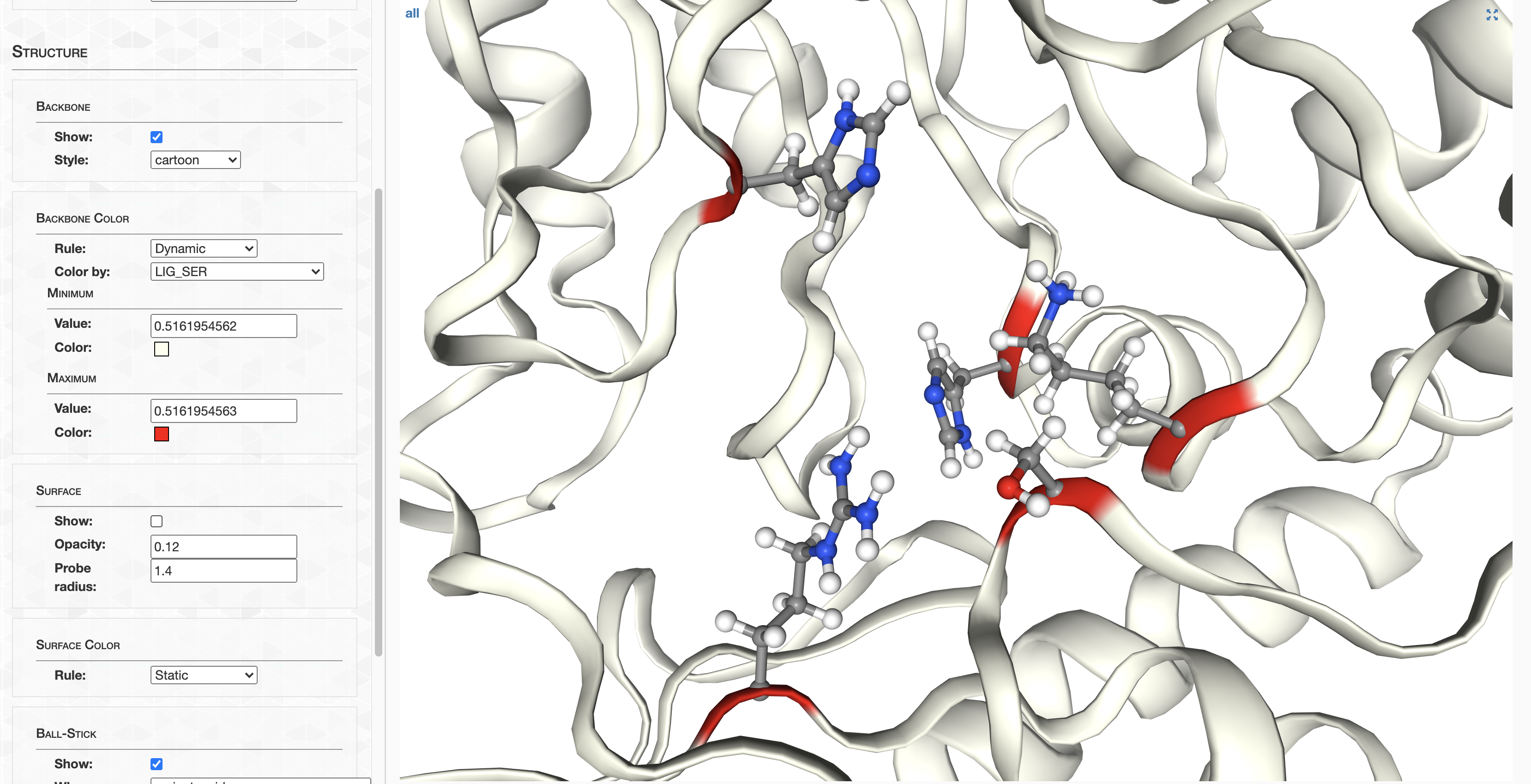
I’ve displayed the sidechains of the reference at these 5 positions.
Anyways, for downstream analyses it will be extremely useful to annotate all of the entries in 11_SCVs.txt pertaining to Gene #1326 with their own special DTL. ZZ_SCRIPTS/append_dist_to_lig.py, the script you just ran, is capable of doing just that after adjusting its runtime parameters slightly:
python ZZ_SCRIPTS/append_dist_to_lig.py --gene 1326 \
                                        --ligand SER \
                                        --save-as-misc-data
anvi-import-misc-data -c CONTIGS.db \
                      -t amino_acids \
                      SER_dist_1326_misc_data.txt
Like before, this generates a misc-data-amino-acids-txt that I imported just for safe keeping.
If you have custom gene-ligand combos you would like to calculate DTL for, you could follow the procedure I just outlined.
Step 14: Calculating pN and pS
If you’re here for a mathematical description of pN and pS–whether it be for per-site, per-group, per-gene calculations, you can find all that in the Methods section of the paper.
Per-site
As mentioned in Step 9, all per-site pN and pS values are appended as columns to the variability-profile, 11_SCVs.txt. That means this data is readily available for you.
If you want to see the underlying code for calculating per-site pN and pS, it can be found in the anvi’o codebase here (click here).
However, there is one small hiccup that I decided to remedy. The problem is the definition of per-site pS:
\[p_N^{(site)} = \frac{1}{n_s} \sum_{c \in C \setminus r} f_c S(c, r) \notag\]where $n_s$ is the number of potential synonymous mutations (see the Methods for a description of all terms). Since Met and Trp both only have 1 codon (ATG and TGG, respectively), $n_s=0$ in these cases. This means whenever the popular consensus is ATG or TGG, there is a division by 0.
There is nothing formally wrong with this, and so anvi-gen-variability-profile respects this division by zero, and sets all per-site pS values to NaN (not-a-number) whenever the reference comparison is ATG or TGG.
However, to me it feels more correct to set per-site pS to 0 in such cases. After all, what is the rate of synonymous polymorphism in these scenarios? Well, there isn’t a rate. It’s zip, zilch–zero, one might even say. And so I set these values accordingly in the following script.
Show/Hide Script
import pandas as pd

df = pd.read_csv('11_SCVs.txt', sep='\t')

# Calculate popular consensus
df['popular_consensus'] = df.\
    groupby('unique_pos_identifier')\
    ['consensus'].\
    transform(lambda x: x.value_counts().index[0])

# If pS_popular_consensus is NaN and popular_consensus is ATG or TGG, set to 0
df.loc[
    (df['popular_consensus'].isin({'ATG', 'TGG'})) & (df['pS_popular_consensus'].isnull()),
    'pS_popular_consensus'
] = 0

# Overwrite
df.to_csv("11_SCVs.txt", sep='\t', index=False)
Command #34
python ZZ_SCRIPTS/fix_nans.py
‣ Time: 30 min
‣ Storage: Minimal
Per-gene
In the field of metagenomics, when people think of pN and pS, they typically think per-gene pN/pS. As such, anvi’o has a dedicated program, anvi-get-pn-ps-ratio, that calculates per-gene pN, pS, and pN/pS.
anvi-get-pn-ps-ratio was developed in conjunction with this study, and has been released as open source software so it may be utilized by the broader community.
anvi-get-pn-ps-ratio takes a SCV variability-profile as input, and churns out a pn-ps-data directory. I named the directory 17_PNPS, and you can run the command as follows:
Command #35
anvi-get-pn-ps-ratio -V 11_SCVs.txt \
                     -c CONTIGS.db \
                     --min-departure-from-consensus 0.04 \
                     --min-coverage 20 \
                     --minimum-num-variants 10 \
                     --comparison popular_consensus \
                     --pivot \
                     -o 17_PNPS
‣ Time: 7 min
‣ Storage: Minimal
The file used extensively in the study is 17_PNPS/pNpS.txt, which is a tabular data form where each row is a different gene, each column is a different sample, and each value is the per-gene pN/pS of a gene in a sample. Here is a preview of the data:
                         ANE_004_05M  ANE_004_40M  ANE_150_05M  ANE_150_40M  ANE_151_05M  ...  RED_32_05M  RED_32_80M  RED_33_05M  RED_34_05M  RED_34_60M
corresponding_gene_call                                                                   ...
1248                        0.024441     0.023470     0.022985     0.022463     0.025215  ...    0.016647    0.019422    0.019010    0.022072    0.026376
1249                        0.078060     0.060345     0.056472     0.066778     0.070270  ...    0.061669    0.076597    0.058939    0.064174    0.053492
1250                        0.012419     0.012937     0.011244     0.012392     0.013154  ...    0.011025    0.015235    0.012687    0.012440    0.015586
1251                        0.018459     0.012003     0.012902     0.012982     0.011404  ...    0.006511    0.010185    0.006364    0.006535    0.013138
1252                        0.058292     0.056371     0.053189     0.052523     0.055640  ...    0.037440    0.044076    0.034135    0.033093    0.042702
...                              ...          ...          ...          ...          ...  ...         ...         ...         ...         ...         ...
2693                        0.037486     0.037132     0.036075     0.041354     0.041974  ...    0.036558    0.036547    0.034810    0.032866    0.039066
2694                        0.050105     0.050185     0.048648     0.047348     0.046988  ...    0.047064    0.049802    0.046035    0.044222    0.050140
2695                        0.046779     0.044541     0.047502     0.045438     0.050766  ...    0.045326    0.053650    0.041775    0.039585    0.043517
2696                        0.089174     0.085332     0.082820     0.083754     0.086197  ...    0.081400    0.081881    0.087031    0.084753    0.083457
2697                        0.058338     0.054560     0.058310     0.055632     0.057657  ...    0.051149    0.057384    0.048692    0.051047    0.051898
Load this sucker up in R or Python to start playing.
library(tidyverse)
df <- read_tsv("17_PNPS/pNpS.txt")
import pandas as pd
df = pd.read_csv('17_PNPS/pNpS.txt', sep='\t')
Per-group (RSA & DTL)
In the study we grouped residues with similar RSA & DTL values and calculated pN and pS not for individual sites or genes, but for different RSA & DTL groups. I wrote a script (are we tired of hearing that yet?) that determines both (1) which group each residue belongs to, and (2) the pN, pS, and pN/pS values of each group. While these metrics can certainly be defined on a per-sample basis, in this analysis samples are concatenated together, producing one pN, pS, and pN/pS value per group.
Here is the rather lengthy script.
Show/Hide Script
#! /usr/bin/env python

import numpy as np
import pandas as pd
import argparse

from pathlib import Path

import anvio.dbops as dbops
import anvio.utils as utils
import anvio.variabilityops as vops

from anvio.tables.miscdata import TableForAminoAcidAdditionalData

ap = argparse.ArgumentParser()
ap.add_argument("-b", "--bins", help="How many bins for each of DTL and RSA? Comma separated to repeat calculation for many bin counts", default='15', type=str)
ap.add_argument("-o", "--output", help="output dir", required=True)
args = ap.parse_args()

# ----------------------------------------------------------------------------------
# Loading databases
# ----------------------------------------------------------------------------------

cdb = dbops.ContigsDatabase('CONTIGS.db')
csc = dbops.ContigsSuperclass(argparse.Namespace(contigs_db='CONTIGS.db'))
csc.init_contig_sequences()

var = vops.VariabilityData(argparse.Namespace(variability_profile='11_SCVs.txt'))

gene_info = cdb.db.get_table_as_dataframe('genes_in_contigs')

# ----------------------------------------------------------------------------------
# Filter by genes of interest
# ----------------------------------------------------------------------------------

# We are only interested in (1) genes with good structure and (2) genes with at least
# 1 predicted ligand binding site. Because ANY_dist is only defined for genes meeting
# this criteria, the most efficient way to subset the data is to filter out any
# entries where ANY_dist is null (NA, NaN, etc.)
var.data = var.data[~var.data['ANY_dist'].isnull()]
goi = var.data['corresponding_gene_call'].unique()

# ----------------------------------------------------------------------------------
# Filter by DTL cutoff
# ----------------------------------------------------------------------------------

# We remove around 8% of residues due their DTL being >40 angstroms. See justification
# in "Calculating distance-to-ligand (DTL)" and Figure S_BIOLIP
var.data = var.data[var.data['ANY_dist'] < 40]

# ----------------------------------------------------------------------------------
# The loop
# ----------------------------------------------------------------------------------

bins = [int(b) for b in args.bins.split(',')]
for bin_count in bins:
    print(f"Working on bin count {bin_count}...")

    # ----------------------------------------------------------------------------------
    # Bin RSA and DTL for each SCV
    # ----------------------------------------------------------------------------------

    # Something somewhat dubious happens here that is worth describing. qcut works by slicing data
    # into different bins, where the bins are not pre-determined widths, but instead are defined
    # dynamically such that each bin contains roughly the same number of datapoints. Now, the issue
    # with this in the case of RSA is that there are _many_ residues with 0 RSA. And so if there are
    # enough requested bins, you could end up with a scenario where the first bin looks like [0,0)
    # and the second _also_ looks like [0,0). This scenario is why the parameter `duplicates`
    # exists. Read more about it here:
    # https://pandas.pydata.org/docs/reference/api/pandas.qcut.html. I have chosen to 'drop' any
    # duplicate any bins, which means the data from both bins gets concatenated together. But a
    # byproduct of this circumstance is that the number of RSA bins will not equal the requested
    # number of bins. Indeed, this is the case in Figure 1, where in fact there are only 13 RSA bins
    # and 15 DTL bins.

    var.data['DTL_group'], DTL_bins = pd.qcut(var.data['ANY_dist'], q=bin_count, duplicates='drop', retbins=True, labels=False)
    var.data['RSA_group'], RSA_bins = pd.qcut(var.data['rel_solvent_acc'], q=bin_count, duplicates='drop', retbins=True, labels=False)

    DTL_bins[0] = np.min(DTL_bins) - np.finfo('float64').eps
    DTL_bins[-1] = np.min(DTL_bins) + 10000
    RSA_bins[0] = np.min(RSA_bins) - np.finfo('float64').eps
    RSA_bins[-1] = np.max(RSA_bins) + np.finfo('float64').eps

    # ----------------------------------------------------------------------------------
    # Get the list of codons for each bin
    #     - This is required in order to calculate the synonymous potential of each bin
    # ----------------------------------------------------------------------------------

    # The easiest way to loop through all the codons in these genes is to take the variability
    # data from a single sample. Since --kiefl-mode was used during the creation of 11_SCVs.txt,
    # every sample has an entry for every codon position. So subsetting 11_SCVs.txt to the entries
    # of a single sample will provide the means to loop through all the codons of all the genes
    # of interest. I randomly decide to pick sample ANE_004_05M, but it actually does not matter.
    coi = [
        'corresponding_gene_call',
        'codon_order_in_gene',
        'DTL_group',
        'RSA_group',
        'reference',
        'ANY_dist',
        'rel_solvent_acc',
    ]
    codon_stats = var.data.loc[var.data['sample_id'] == 'ANE_004_05M', coi]

    max_DTL = 0
    codon_lists = {(x, y):[] for x in range(len(RSA_bins)-1) for y in range(len(DTL_bins)-1)}
    for gene_id in goi:
        gene_codon_stats = codon_stats[codon_stats['corresponding_gene_call'] == gene_id]
        for _, row in gene_codon_stats.iterrows():
            DTL = row['ANY_dist']
            RSA = row['rel_solvent_acc']
            codon = row['reference']

            RSA_bin = np.digitize(RSA, RSA_bins) - 1
            DTL_bin = np.digitize(DTL, DTL_bins) - 1
            codon_lists[(RSA_bin, DTL_bin)].append(codon)

            if DTL > max_DTL:
                max_DTL = DTL

    if any([len(x)==0 for x in codon_lists.values()]):
        print(f"    Some groups have no data. Skipping output for bin count {bin_count}")
        continue

    # ----------------------------------------------------------------------------------
    # Calculate synonymous potentials
    # ----------------------------------------------------------------------------------

    potential_lookups = {}
    for key, codon_list in codon_lists.items():
        potential_lookups[key] = utils.get_synonymous_and_non_synonymous_potential(codon_list, just_do_it=True)[:2]
    potentials = np.transpose(np.array(list(zip(*var.data[['RSA_group', 'DTL_group']].apply(lambda row: potential_lookups[tuple(row.tolist())], axis=1).values))))

    # ----------------------------------------------------------------------------------
    # Churn out pN/pS, pS, and pN
    # ----------------------------------------------------------------------------------

    var.calc_pN_pS(grouping='DTL_RSA', comparison='popular_consensus', potentials=potentials)
    n_samples = var.data['sample_id'].nunique()
    pN = var.data.groupby(['DTL_group', 'RSA_group'])['pN_DTL_RSA_popular_consensus'].sum()/n_samples
    pS = var.data.groupby(['DTL_group', 'RSA_group'])['pS_DTL_RSA_popular_consensus'].sum()/n_samples
    pNpS = pN/pS

    pN = pN.reset_index()
    pS = pS.reset_index()
    pNpS = pNpS.reset_index()

    DTL_bins[-1] = max_DTL + np.finfo('float64').eps

    pNpS['DTL'] = pNpS['DTL_group'].apply(lambda group: DTL_bins[group])
    pN['DTL'] = pN['DTL_group'].apply(lambda group: DTL_bins[group])
    pS['DTL'] = pS['DTL_group'].apply(lambda group: DTL_bins[group])

    pNpS['DTL_range'] = pNpS['DTL_group'].apply(lambda group: '[' + str(abs(np.round(DTL_bins[group], 1))) + ',' + str(abs(np.round(DTL_bins[group+1], 1))) + ')')
    pN['DTL_range'] = pN['DTL_group'].apply(lambda group: '[' + str(abs(np.round(DTL_bins[group], 1))) + ',' + str(abs(np.round(DTL_bins[group+1], 1))) + ')')
    pS['DTL_range'] = pS['DTL_group'].apply(lambda group: '[' + str(abs(np.round(DTL_bins[group], 1))) + ',' + str(abs(np.round(DTL_bins[group+1], 1))) + ')')

    pNpS['RSA'] = pNpS['RSA_group'].apply(lambda group: RSA_bins[group])
    pN['RSA'] = pN['RSA_group'].apply(lambda group: RSA_bins[group])
    pS['RSA'] = pS['RSA_group'].apply(lambda group: RSA_bins[group])

    pNpS['RSA_range'] = pNpS['RSA_group'].apply(lambda group: '[' + str(np.abs(np.round(RSA_bins[group], 2))) + ',' + str(np.abs(np.round(RSA_bins[group+1], 2))) + ')')
    pN['RSA_range'] = pN['RSA_group'].apply(lambda group: '[' + str(np.abs(np.round(RSA_bins[group], 2))) + ',' + str(np.abs(np.round(RSA_bins[group+1], 2))) + ')')
    pS['RSA_range'] = pS['RSA_group'].apply(lambda group: '[' + str(np.abs(np.round(RSA_bins[group], 2))) + ',' + str(np.abs(np.round(RSA_bins[group+1], 2))) + ')')

    pN['s_sites'] = pN.apply(lambda row: potential_lookups[row['RSA_group'], row['DTL_group']][0], axis=1)
    pN['ns_sites'] = pN.apply(lambda row: potential_lookups[row['RSA_group'], row['DTL_group']][1], axis=1)
    pS['s_sites'] = pS.apply(lambda row: potential_lookups[row['RSA_group'], row['DTL_group']][0], axis=1)
    pS['ns_sites'] = pS.apply(lambda row: potential_lookups[row['RSA_group'], row['DTL_group']][1], axis=1)
    pNpS['s_sites'] = pNpS.apply(lambda row: potential_lookups[row['RSA_group'], row['DTL_group']][0], axis=1)
    pNpS['ns_sites'] = pNpS.apply(lambda row: potential_lookups[row['RSA_group'], row['DTL_group']][1], axis=1)

    # ----------------------------------------------------------------------------------
    # Write to directory
    # ----------------------------------------------------------------------------------

    output_dir = Path(args.output)
    output_dir.mkdir(exist_ok=True)
    pNpS.rename(columns={0: 'pNpS_DTL_RSA_popular_consensus'}).to_csv(output_dir/f'pNpS_{bin_count}.txt', sep='\t', index=False)
    pN.to_csv(output_dir/f'pN_{bin_count}.txt', sep='\t', index=False)
    pS.to_csv(output_dir/f'pS_{bin_count}.txt', sep='\t', index=False)

    var.data.groupby(['DTL_group', 'RSA_group']).size().reset_index().rename(columns={0: 'count'}).to_csv(output_dir/f'counts_{bin_count}.txt', sep='\t', index=False)
Go ahead and run the thing.
Command #36
python ZZ_SCRIPTS/analysis_pnps_d_and_rsa.py -b 15 \
                                             -o 17_PNPS_RSA_AND_DTL
‣ Time: 25 min
‣ Storage: Minimal
-b indicates to the number of bins for each variable. I chose 15, but in Figure SI4 I do a whole range of bin values and show how the linear regressions of pN vary with respect to bin size.
The output for all of the results is in 17_PNPS_RSA_AND_DTL.
The bin widths are determined by looking at the marginal distributions of RSA and DTL, and creating bins of each quantile. The rationale behind this decision came from wanting to create roughly equal group sizes, since RSA and DTL are in no way uniformly distributed. While creating a grid of equal sized groups is no problem with a 1D distribution (e.g. just RSA, or just DTL), it is impossible to create a grid of equal sized groups with a 2D distribution (in this case, with variables RSA and DTL). The best solution I could come up with was to create bin widths of each dimension by marginalizing over the dimension.
You can view the bin ranges and their sizes in 17_PNPS_RSA_AND_DTL/counts_15.txt:
| DTL_group | RSA_group | count |
|---|---|---|
| 0 | 0 | 183964 |
| 0 | 1 | 72890 |
| 0 | 2 | 84138 |
| 0 | 3 | 79254 |
| 0 | 4 | 65120 |
| 0 | 5 | 57128 |
| 0 | 6 | 49580 |
| 0 | 7 | 39368 |
| 0 | 8 | 34780 |
| 0 | 9 | 28786 |
| 0 | 10 | 29008 |
| 0 | 11 | 24642 |
| 0 | 12 | 18426 |
| 1 | 0 | 260850 |
| 1 | 1 | 76516 |
| 1 | 2 | 61272 |
| 1 | 3 | 57276 |
| 1 | 4 | 51874 |
| 1 | 5 | 45880 |
| (…) | (…) | (…) |
And as you would expect, you can also find $pN^{(site)}$, $pS^{(site)}$, and $pN/pS^{(site)}$ in 17_PNPS_RSA_AND_DTL. Here is $pN/pS^{(site)}$:
| DTL_group | RSA_group | pNpS_DTL_RSA_popular_consensus | DTL | DTL_range | RSA | RSA_range | s_sites | ns_sites |
|---|---|---|---|---|---|---|---|---|
| 0 | 0 | 0.013870655291934623 | -2.220446049250313e-16 | [0.0,3.9) | -2.220446049250313e-16 | [0.0,0.01) | 1795.9999999998709 | 5638.000000000129 |
| 0 | 1 | 0.011526765560231033 | -2.220446049250313e-16 | [0.0,3.9) | 0.01140684410646388 | [0.01,0.03) | 643.0000000000032 | 2329.999999999997 |
| 0 | 2 | 0.010713124094289164 | -2.220446049250313e-16 | [0.0,3.9) | 0.03157894736842105 | [0.03,0.07) | 716.3333333333449 | 2655.666666666655 |
| 0 | 3 | 0.0081719865439211 | -2.220446049250313e-16 | [0.0,3.9) | 0.06598984771573604 | [0.07,0.11) | 687.3333333333416 | 2549.6666666666583 |
| 0 | 4 | 0.014303815347239306 | -2.220446049250313e-16 | [0.0,3.9) | 0.10833333333333334 | [0.11,0.16) | 552.999999999993 | 2096.0000000000073 |
| 0 | 5 | 0.014199467540218183 | -2.220446049250313e-16 | [0.0,3.9) | 0.15833333333333333 | [0.16,0.22) | 494.666666666656 | 1824.333333333344 |
| 0 | 6 | 0.019434217438879717 | -2.220446049250313e-16 | [0.0,3.9) | 0.2153846153846154 | [0.22,0.28) | 395.3333333333283 | 1596.6666666666717 |
| 0 | 7 | 0.028759770102374054 | -2.220446049250313e-16 | [0.0,3.9) | 0.2774193548387097 | [0.28,0.34) | 352.33333333333076 | 1267.6666666666692 |
| 0 | 8 | 0.03467296319572384 | -2.220446049250313e-16 | [0.0,3.9) | 0.3390804597701149 | [0.34,0.4) | 278.00000000000165 | 1110.9999999999984 |
| 0 | 9 | 0.04649300749307973 | -2.220446049250313e-16 | [0.0,3.9) | 0.40384615384615385 | [0.4,0.48) | 227.66666666666876 | 954.3333333333312 |
| 0 | 10 | 0.032357307132775646 | -2.220446049250313e-16 | [0.0,3.9) | 0.4766839378238342 | [0.48,0.56) | 224.66666666666868 | 945.3333333333313 |
| 0 | 11 | 0.06822789757258542 | -2.220446049250313e-16 | [0.0,3.9) | 0.559322033898305 | [0.56,0.67) | 184.00000000000085 | 820.9999999999991 |
| 0 | 12 | 0.07601265475140384 | -2.220446049250313e-16 | [0.0,3.9) | 0.6735751295336787 | [0.67,1.0) | 138.99999999999957 | 614.0000000000005 |
| 1 | 0 | 0.01516724399039351 | 3.860591173171997 | [3.9,6.1) | -2.220446049250313e-16 | [0.0,0.01) | 2688.333333333438 | 7874.666666666562 |
| 1 | 1 | 0.015082762407656826 | 3.860591173171997 | [3.9,6.1) | 0.01140684410646388 | [0.01,0.03) | 744.333333333348 | 2369.666666666652 |
| 1 | 2 | 0.01289258431373061 | 3.860591173171997 | [3.9,6.1) | 0.03157894736842105 | [0.03,0.07) | 574.9999999999955 | 1882.0000000000045 |
| 1 | 3 | 0.01770026803304325 | 3.860591173171997 | [3.9,6.1) | 0.06598984771573604 | [0.07,0.11) | 544.3333333333253 | 1783.6666666666747 |
| 1 | 4 | 0.020790495565182615 | 3.860591173171997 | [3.9,6.1) | 0.10833333333333334 | [0.11,0.16) | 481.99999999999005 | 1636.00000000001 |
| 1 | 5 | 0.024905304363086384 | 3.860591173171997 | [3.9,6.1) | 0.15833333333333333 | [0.16,0.22) | 395.3333333333283 | 1455.6666666666717 |
| (…) | (…) | (…) | (…) | (…) | (…) | (…) | (…) | (…) |
Step 15: Codon properties
You should follow this step to ensure reproducibility for any downstream steps that expect this data to be present, but during revisions we’ve lost confidence in our codon rarity analysis and have removed it from the paper.
In the paper, we measured how codon usage varies from sample-to-sample, ultimately illustrating that rare codons are preferred in structurally/functionally noncritical sites. First, let’s go through the different definitions of rarity.
Definitions of rarity
First and foremost, when the paper discusses rarity, it is always, always, always referring to synonymous codon rarity, which I’ll define in just a second. I mention this because in the files and scripts below, you will find other definitions of rarity that I experimented with during the exploratory phase of this study. Since they are interesting in their own right, I have kept them here so that you too can experiment with them. However, the paper is concerned specifically with synonymous codon rarity.
Synonymous codon rarity
Synonymous codon rarity describes how rare a codon is in the HIMB83 genome relative to other codons that encode the same amino acid. Mathematically, the synonymous codon rarity of codon $i$ is
\[R_{i} = 1 - \frac {f_i} {\sum_j S(i, j) \, f_j}\]where $f_{i}$ is the proportion of codons in the HIMB83 genome that are the $i$th codon, and where $S(i, j)$ is the indicator function
\[S(i, j) = 1 \, if \, synonymous(i, j) \, else \, 0\](Mathematically, we are assuming codon $i$ is synonymous with itself)
As an example, what is the synonymous codon rarity of GCC, which encodes the amino acid alanine? First, we count all of the instances of GCC in the codons of HIMB83 (all 1470 coding genes) and divide it by the number of codons in HIMB83. That number is $f_{GCC}$. Then we do the same thing for all alanine codons, GCA, GCC, GCG, and GCT. We are thus left with
\[\displaylines{f_{GCA} = 0.02553 \\ f_{GCC} = 0.00329 \\ f_{GCG} = 0.00294 \\ f_{GCT} = 0.0232}\]What we are looking at here are the frequencies of alanine codons relative to all codons. For example, this says that 0.329% of codons in the HIMB83 genome are GCC. To calculate synonymous codon rarity, we apply the above formula:
\[R_{GCC} = 1 - \frac {0.00329} {0.02553 + 0.00329 + 0.00294 + 0.0232} = 0.94\]Since GCC occurs much less frequently than its synonymous counterparts GCA and GCT, it gets a high synonymous codon rarity score of 0.94.
Codon rarity
Codon rarity is similar to synonymous codon rarity, except values are not normalized by codons sharing the same amino acid. It is calculated in two parts. First, the unnormalized codon rarity for each codon $i$ is calculated as
\[R'_{i}=1-f_i\]where $f_i$ is the frequency that a codon was observed in the HIMB83 genome sequence. Then, $R’_{i}$ is normalized such that the codons with the lowest and highest values get rarity scores of 0 and 1, respectively:
\[R_i = \frac{R'_i-\min(R')}{\max(R'_{i})-\min(R')},\]where $\min(R’)$ and $\max(R’)$ correspond to the smallest and largest unnormalized rarity scores.
This metric can be useful for assessing how rare a codon is relative to all codons, not just relative to those it is synonymous with.
Amino acid rarity
Amino acid rarity is just the same as codon rarity, except instead of comparing amino acids, we are comparing amino acids. First, the unnormalized codon rarity for each codon $i$ is calculated as
\[R'_{i}=1-f_i\]where $f_i$ is the frequency that a codon was observed in the HIMB83 genome sequence. Then, $R’_{i}$ is normalized such that the codons with the lowest and highest values get rarity scores of 0 and 1, respectively:
\[R_i = \frac{R'_i-\min(R')}{\max(R'_{i})-\min(R')},\]where $\min(R’)$ and $\max(R’)$ correspond to the smallest and largest unnormalized rarity scores.
This metric can be useful for assessing how rare amino acids are relative to each other.
Calculating rarity
To calculate metrics such as rarity for codons and amino acids, I created the script ZZ_SCRIPTS/get_codon_trna_composition.sh.
Show/Hide Script
Here is ZZ_SCRIPTS/get_codon_trna_composition.sh:
#! /usr/bin/env bash

anvi-get-codon-frequencies -c CONTIGS.db \
                           -o codon_freqs.txt \
                           --collapse \
                           --percent-normalize

anvi-get-codon-frequencies -c CONTIGS.db \
                           -o codon_freqs_synonymous.txt \
                           --collapse \
                           --merens-codon-normalization

anvi-get-codon-frequencies -c CONTIGS.db \
                           -o aa_freqs.txt \
                           --collapse \
                           --percent-normalize \
                           --return-AA-frequencies-instead

anvi-scan-trnas -c CONTIGS.db -T 6 --trna-cutoff-score 20 --just-do-it
anvi-get-sequences-for-hmm-hits -c CONTIGS.db --hmm-source Transfer_RNAs -o trnas.fa

python ZZ_SCRIPTS/get_codon_trna_composition.py
Here is the script ZZ_SCRIPTS/get_codon_trna_composition.py, which it calls upon.
#! /usr/bin/env python

import pandas as pd
import anvio.utils as utils
import anvio.fastalib as u
import anvio.constants as constants

from collections import Counter

fasta = u.SequenceSource('trnas.fa')

codon_count = {
    'codon': [c for c in constants.codons],
    'anticodon': [utils.rev_comp(c) for c in constants.codons],
    'amino_acid': [constants.codon_to_AA[c] for c in constants.codons],
    'GC_fraction': [sum([v for k, v in Counter(c).items() if k in ('G', 'C')])/3 for c in constants.codons],
    'trna_copy_number': [0] * len(constants.codons)
}

while next(fasta):
    aa, anticodon = fasta.id.split('_')[:2]
    codon = utils.rev_comp(anticodon)
    index = codon_count['codon'].index(codon)
    codon_count['trna_copy_number'][index] += 1

df = pd.DataFrame(codon_count)

# ------------------------------------------------------------------------------------------------------
# Calculate codon rarity. This is calculated from codon frequencies that sum to 1
# ------------------------------------------------------------------------------------------------------

codon_freq = pd.read_csv('codon_freqs.txt', sep='\t').T.reset_index().tail(-1).rename(columns={0: 'freq', 'index': 'codon'})
codon_freq['amino_acid'] = codon_freq['codon'].map(lambda codon: codon_count['amino_acid'][codon_count['codon'].index(codon)])
codon_freq['rarity'] = 100-codon_freq['freq']
# normalize rarity between 0 and 1
M, m = codon_freq['rarity'].max(), codon_freq['rarity'].min()
codon_freq['rarity'] = (codon_freq['rarity'] - m) / (M - m)

# ------------------------------------------------------------------------------------------------------
# Calculate codon rarity per AA. This is calculated from codon frequencies that sum to 1 for each AA
# and is called "synonymous rarity"
# ------------------------------------------------------------------------------------------------------

codon_freq_per_aa = pd.read_csv('codon_freqs_synonymous.txt', sep='\t').T.reset_index().tail(-1).rename(columns={0: 'freq_per_aa'})
codon_freq_per_aa[['amino_acid', 'codon']] = codon_freq_per_aa['index'].str.split('-', expand=True)
codon_freq_per_aa.drop('index', axis=1, inplace=True)
codon_freq_per_aa['syn_rarity'] = (100-codon_freq_per_aa['freq_per_aa'])/100

# ------------------------------------------------------------------------------------------------------
# Calculate amino acid rarity. This is calculated from amino acid frequencies that sum to 1
# ------------------------------------------------------------------------------------------------------

aa_freq = pd.read_csv('aa_freqs.txt', sep='\t').T.reset_index().tail(-1).rename(columns={0: 'aa_freq', 'index': 'amino_acid'})
aa_freq['aa_rarity'] = 100-aa_freq['aa_freq']
# normalize rarity between 0 and 1
M, m = aa_freq['aa_rarity'].max(), aa_freq['aa_rarity'].min()
aa_freq['aa_rarity'] = (aa_freq['aa_rarity'] - m) / (M - m)

# ------------------------------------------------------------------------------------------------------
# Merge
# ------------------------------------------------------------------------------------------------------

df = df.\
    merge(codon_freq, how='left', on=['codon', 'amino_acid']).\
    merge(codon_freq_per_aa, how='left', on=['codon', 'amino_acid']).\
    merge(aa_freq, how='left', on=['amino_acid']).\
    sort_values(by='amino_acid')

# ------------------------------------------------------------------------------------------------------
# Add the atomic composition
# ------------------------------------------------------------------------------------------------------

atoms = constants.AA_atomic_composition
atoms['STP'] = Counter()

df['N'] = df['amino_acid'].map(lambda x: atoms[x]['N'])
df['C'] = df['amino_acid'].map(lambda x: atoms[x]['C'])
df['O'] = df['amino_acid'].map(lambda x: atoms[x]['O'])
df['S'] = df['amino_acid'].map(lambda x: atoms[x]['S'])

# based on the available tRNA genes we construct this putative association between codons and the
# the tRNA anticodons that decode them. This was done by hand.
codon_to_decoder = dict(
    GCA = 'TGC',
    GCC = 'TGC',
    GCG = 'TGC',
    GCT = 'TGC',
    CGA = 'TCG',
    CGC = 'TCG',
    CGG = 'TCG',
    CGT = 'TCG',
    AGA = 'TCT',
    AGG = 'TCT',
    AAT = 'GTT',
    AAC = 'GTT',
    GAT = 'GTC',
    GAC = 'GTC',
    TGT = 'GCA',
    TGC = 'GCA',
    CAA = 'TTG',
    CAG = 'TTG',
    GAA = 'TTC',
    GAG = 'TTC',
    GGT = 'GCC',
    GGC = 'GCC',
    GGA = 'TCC',
    GGG = 'TCC',
    CAT = 'GTG',
    CAC = 'GTG',
    ATT = 'GAT',
    ATC = 'GAT',
    ATA = 'CAT',
    TTG = 'CAA',
    TTA = 'TAA',
    CTA = 'TAG',
    CTC = 'TAG',
    CTG = 'TAG',
    CTT = 'TAG',
    AAA = 'TTT',
    AAG = 'TTT',
    ATG = 'CAT',
    TTT = 'GAA',
    TTC = 'GAA',
    CCA = 'TGG',
    CCC = 'TGG',
    CCG = 'TGG',
    CCT = 'TGG',
    AGT = 'GCT',
    AGC = 'GCT',
    TCT = 'GGA',
    TCC = 'GGA',
    TCA = 'TGA',
    TCG = 'TGA',
    ACC = 'GGT',
    ACT = 'GGT',
    ACA = 'TGT',
    ACG = 'TGT',
    TGG = 'CCA',
    TAT = 'GTA',
    TAC = 'GTA',
    GTT = 'GAC',
    GTC = 'GAC',
    GTA = 'TAC',
    GTG = 'TAC',
)

df['trna'] = df['codon'].map(codon_to_decoder)

df.to_csv("codon_trna_composition.txt", sep='\t', index=False)
When you’re ready (it just takes a couple seconds), run it:
Command #37
bash ZZ_SCRIPTS/get_codon_trna_composition.sh
‣ Time: <1 min
‣ Storage: Minimal
This script utilizes anvi-get-codon-frequencies, anvi-scan-trnas, anvi-get-sequences-for-hmm-hits, and some Python in order to produce the following files:
codon_freqs.txt
codon_freqs_synonymous.txt
codon_trna_composition.txt
codon_freqs.txt and is produced by anvi-get-codon-frequencies and compiles the percentage of total codons found in the HIMB83 genome that correspond to each codon:
| gene_callers_id | GCA | GCC | GCG | GCT | AGA | AGG | CGA | CGC | CGG | CGT | AAC | AAT | GAC | GAT | TGC | TGT | CAA | CAG | GAA | GAG | GGA | GGC | GGG | GGT | CAC | CAT | ATA | ATC | ATT | CTA | CTC | CTG | CTT | TTA | TTG | AAA | AAG | ATG | TTC | TTT | CCA | CCC | CCG | CCT | TAA | TAG | TGA | AGC | AGT | TCA | TCC | TCG | TCT | ACA | ACC | ACG | ACT | TGG | TAC | TAT | GTA | GTC | GTG | GTT |
|---|---|---|---|---|---|---|---|---|---|---|---|---|---|---|---|---|---|---|---|---|---|---|---|---|---|---|---|---|---|---|---|---|---|---|---|---|---|---|---|---|---|---|---|---|---|---|---|---|---|---|---|---|---|---|---|---|---|---|---|---|---|---|---|---|
| all | 2.553 | 0.329 | 0.294 | 2.32 | 2.606 | 0.243 | 0.174 | 0.015 | 0.017 | 0.144 | 1.269 | 5.375 | 0.872 | 4.344 | 0.193 | 0.771 | 2.235 | 0.404 | 4.811 | 1.337 | 2.685 | 0.497 | 0.373 | 2.628 | 0.362 | 1.239 | 3.073 | 0.887 | 5.51 | 0.928 | 0.169 | 0.193 | 1.641 | 5.397 | 1.039 | 9.209 | 1.243 | 2.203 | 0.667 | 4.684 | 1.695 | 0.16 | 0.133 | 1.259 | 0.242 | 0.041 | 0.043 | 0.457 | 1.455 | 2.39 | 0.223 | 0.23 | 2.053 | 2.114 | 0.375 | 0.212 | 2.019 | 0.938 | 0.735 | 2.721 | 1.88 | 0.303 | 0.419 | 2.973 |
These can be used to calculate codon rarity.
Similary, codon_freqs_synonymous.txt is also produced by anvi-get-codon-frequencies but compiles the relative percentages of codons for a given amino acid. It looks like this:
| gene_callers_id | Ala-GCA | Ala-GCC | Ala-GCG | Ala-GCT | Arg-AGA | Arg-AGG | Arg-CGA | Arg-CGC | Arg-CGG | Arg-CGT | Asn-AAC | Asn-AAT | Asp-GAC | Asp-GAT | Cys-TGC | Cys-TGT | Gln-CAA | Gln-CAG | Glu-GAA | Glu-GAG | Gly-GGA | Gly-GGC | Gly-GGG | Gly-GGT | His-CAC | His-CAT | Ile-ATA | Ile-ATC | Ile-ATT | Leu-CTA | Leu-CTC | Leu-CTG | Leu-CTT | Leu-TTA | Leu-TTG | Lys-AAA | Lys-AAG | Met-ATG | Phe-TTC | Phe-TTT | Pro-CCA | Pro-CCC | Pro-CCG | Pro-CCT | STP-TAA | STP-TAG | STP-TGA | Ser-AGC | Ser-AGT | Ser-TCA | Ser-TCC | Ser-TCG | Ser-TCT | Thr-ACA | Thr-ACC | Thr-ACG | Thr-ACT | Trp-TGG | Tyr-TAC | Tyr-TAT | Val-GTA | Val-GTC | Val-GTG | Val-GTT |
|---|---|---|---|---|---|---|---|---|---|---|---|---|---|---|---|---|---|---|---|---|---|---|---|---|---|---|---|---|---|---|---|---|---|---|---|---|---|---|---|---|---|---|---|---|---|---|---|---|---|---|---|---|---|---|---|---|---|---|---|---|---|---|---|---|
| all | 46.46 | 5.98 | 5.345 | 42.215 | 81.442 | 7.591 | 5.445 | 0.479 | 0.535 | 4.508 | 19.093 | 80.907 | 16.72 | 83.28 | 19.995 | 80.005 | 84.685 | 15.315 | 78.259 | 21.741 | 43.425 | 8.044 | 6.027 | 42.504 | 22.631 | 77.369 | 32.448 | 9.364 | 58.188 | 9.907 | 1.808 | 2.057 | 17.516 | 57.62 | 11.091 | 88.111 | 11.889 | 100.0 | 12.457 | 87.543 | 52.21 | 4.94 | 4.085 | 38.764 | 74.268 | 12.457 | 13.274 | 6.717 | 21.379 | 35.105 | 3.274 | 3.372 | 30.153 | 44.792 | 7.941 | 4.49 | 42.777 | 100.0 | 21.256 | 78.744 | 33.724 | 5.437 | 7.509 | 53.33 |
These can be used to calculated synonymous codon rarity, which in the paper we oftentimes refer to it simply as ‘rarity’.
The third output, codon_trna_composition.txt, summarizes several pieces of information about each codon, such as the corresponding amino acid, the number of cognate tRNA genes found in HIMB83, as well as metrics like the frequency that its found in the genome, including the synonymous codon rarity metric used in the paper. Here it is:
| codon | anticodon | amino_acid | GC_fraction | trna_copy_number | freq | rarity | freq_per_aa | syn_rarity | aa_freq | aa_rarity | N | C | O | S | trna |
|---|---|---|---|---|---|---|---|---|---|---|---|---|---|---|---|
| GCC | GGC | Ala | 1.0 | 0 | 0.32899999999999996 | 0.9658472917119868 | 5.98 | 0.9401999999999999 | 5.496 | 0.48938271604938255 | 1 | 3 | 2 | 0 | TGC |
| GCT | AGC | Ala | 0.6666666666666666 | 0 | 2.32 | 0.7492930171851216 | 42.215 | 0.57785 | 5.496 | 0.48938271604938255 | 1 | 3 | 2 | 0 | TGC |
| GCG | CGC | Ala | 1.0 | 0 | 0.294 | 0.9696541222536441 | 5.345 | 0.94655 | 5.496 | 0.48938271604938255 | 1 | 3 | 2 | 0 | TGC |
| GCA | TGC | Ala | 0.6666666666666666 | 1 | 2.553 | 0.723950402436372 | 46.46 | 0.5354 | 5.496 | 0.48938271604938255 | 1 | 3 | 2 | 0 | TGC |
| AGA | TCT | Arg | 0.3333333333333333 | 1 | 2.6060000000000003 | 0.7181857733304337 | 81.442 | 0.18558000000000008 | 3.199 | 0.7162469135802465 | 4 | 6 | 2 | 0 | TCT |
| CGC | GCG | Arg | 1.0 | 0 | 0.015 | 1.0 | 0.479 | 0.99521 | 3.199 | 0.7162469135802465 | 4 | 6 | 2 | 0 | TCG |
| CGA | TCG | Arg | 0.6666666666666666 | 1 | 0.174 | 0.9827061126821833 | 5.445 | 0.9455500000000001 | 3.199 | 0.7162469135802465 | 4 | 6 | 2 | 0 | TCG |
| CGG | CCG | Arg | 1.0 | 0 | 0.017 | 0.9997824668261915 | 0.535 | 0.99465 | 3.199 | 0.7162469135802465 | 4 | 6 | 2 | 0 | TCG |
| CGT | ACG | Arg | 0.6666666666666666 | 1 | 0.14400000000000002 | 0.9859691102893186 | 4.508 | 0.95492 | 3.199 | 0.7162469135802465 | 4 | 6 | 2 | 0 | TCG |
| (…) | (…) | (…) | (…) | (…) | (…) | (…) | (…) | (…) | (…) | (…) | (…) | (…) | (…) | (…) | (…) |
As you can see, it is basically a one-stop shop for all your codon property needs.
Adding synonymous codon rarity to SCV data
Just like RSA and DTL, codon rarity is a metric that we definitely want associated to each SCV (row) in the variability-profile, 11_SCVs.txt. This is the last piece of information we’ll add to the 11_SCVs.txt.
Show/Hide Script
import numpy as np
import pandas as pd
import argparse
import anvio.constants as constants
import anvio.variabilityops as vops

aa_variability_profile = '10_SAAVs.txt'
print('loading saavs table')
aa_var = vops.VariabilityData(argparse.Namespace(variability_profile=aa_variability_profile))
print('converting table to frequencies')
aa_var.convert_counts_to_frequencies(retain_counts=True)

amino_acids = constants.amino_acids
col_names = [aa + '_freq' for aa in amino_acids]

df = pd.read_csv('codon_trna_composition.txt', sep='\t').sort_values('amino_acid')
aa_rarity_array = df[['aa_rarity', 'amino_acid']].drop_duplicates()['aa_rarity'].values

print('calculating aa_rarity')
aa_var.data['aa_rarity'] = np.sum(aa_var.data[col_names].values*aa_rarity_array, axis=1)

print('dropping frequency columns')
# Do not hold onto the frequency columns
aa_var.data.drop(col_names, axis=1, inplace=True)

print('saving aa table')
aa_var.data.to_csv(aa_variability_profile, sep='\t', index=False)

# -----------------------------------

variability_profile = '11_SCVs.txt'
print('loading table')
var = vops.VariabilityData(argparse.Namespace(variability_profile=variability_profile))
print('converting table to frequencies')
var.convert_counts_to_frequencies(retain_counts=True)

codons = constants.codons
coding_codons = constants.coding_codons
col_names = [codon + '_freq' for codon in codons]
coding_col_names = [codon + '_freq' for codon in coding_codons]

df = pd.read_csv('codon_trna_composition.txt', sep='\t').sort_values('codon')
rarity_array = df.rarity.values
syn_rarity_array = df.syn_rarity.values
aa_rarity = df.aa_rarity.values
GC_fraction = df.GC_fraction.values

print('calculating codon_rarity')
var.data['codon_rarity'] = np.sum(var.data[col_names].values*rarity_array, axis=1)
print('calculating syn_codon_rarity')
var.data['syn_codon_rarity'] = np.sum(var.data[col_names].values*syn_rarity_array, axis=1)
print('calculating aa_rarity')
var.data['aa_rarity'] = np.sum(var.data[col_names].values*aa_rarity, axis=1)
print('calculating GC_fraction')
var.data['GC_fraction'] = np.sum(var.data[col_names].values*GC_fraction, axis=1)

# -----------------------------------

print('dropping frequency columns')
# Do not hold onto the frequency columns
var.data.drop(col_names, axis=1, inplace=True)

print('saving table')
var.data.to_csv(variability_profile, sep='\t', index=False)
Command #38
python ZZ_SCRIPTS/append_codon_trna_composition.py
‣ Time: 32 min
‣ Storage: 750 Mb
This script does a bit more than I’m letting on, because it adds codon rarity, synonymous codon rarity, and amino acid rarity as columns to our variability-profile 11_SCVs.txt, as well as amino acid rarity as a column to our variability-profile 10_SAAVs.txt.
Step 16: Breathe
Okay. If you’ve made it this far, this marks the end of this chapter, and subsequently the end of the data processing workflow. We started from nothing but the internet, and we have built up the totality of data we will need for all subsequent analyses, which are carried out in the next chapter. We have just invested an enormous amount of work and forethought that we will now be able to stand upon in order to harvest the fruits of our labour.
See you in the next chapter.
Aux. Step 1: Pangenome detour
This is the first (and potentially only) auxiliary step, meaning it is not required for the central analyses of this paper. For this reason, you can skip this step if you want.
But if you’re reading this, you’ve more than likely beeen redirected to this section of the workflow, because the analysis you’re interested in requires this step to be completed. In that case, you’re in the right place.
How does the gene content differ between HIMB83 and the other 20 genomes? What genes are present and absent, what is the percent similarity of the homologs? What is the average nucleotide identity (ANI) of these genomes to HIMB83?
These questions all fall under the umbrella of pangenomics, and since we now have contigs-dbs for each genome (in 07_SPLIT/), we are in the perfect position for a quick detour into the land of pangenomics. While a detour, this is required for some supplemental figures down the road.
In this paper I made 2 pangenomes. One compares all 21 SAR11 genomes to one another, and the other compares HIMB83 to its closest relative in this genome collection, HIMB122.
To create this 2 pangenomes, I created a bash script called ZZ_SCRIPTS/make_pangenomes.sh.
Show/Hide Script
#! /usr/bin/env bash

# Delete all previous pangenomes
rm -rf 07_PANGENOME*
rm -rf 07_SUMMARY_PAN*

mkdir 07_PANGENOME
mkdir 07_PANGENOME_COMP_TO_HIMB122

python ZZ_SCRIPTS/gen_external_genomes_file.py

# Full pangeome
anvi-gen-genomes-storage -e 07_EXTERNAL_GENOMES.txt -o 07_PANGENOME/SAR11-GENOMES.db
anvi-pan-genome -g 07_PANGENOME/SAR11-GENOMES.db -n SAR11 -o 07_PANGENOME/PANGENOME -T $1
anvi-script-add-default-collection -p 07_PANGENOME/PANGENOME/SAR11-PAN.db
anvi-summarize -p 07_PANGENOME/PANGENOME/SAR11-PAN.db -g 07_PANGENOME/SAR11-GENOMES.db -C DEFAULT -o 07_SUMMARY_PAN
gzip -d 07_SUMMARY_PAN/SAR11_gene_clusters_summary.txt.gz

# HIMB122
anvi-gen-genomes-storage -e 07_EXTERNAL_GENOMES_COMP_TO_HIMB122.txt -o 07_PANGENOME_COMP_TO_HIMB122/SAR11-GENOMES.db
anvi-pan-genome -g 07_PANGENOME_COMP_TO_HIMB122/SAR11-GENOMES.db -n SAR11 -o 07_PANGENOME_COMP_TO_HIMB122/PANGENOME -T $1
anvi-script-add-default-collection -p 07_PANGENOME_COMP_TO_HIMB122/PANGENOME/SAR11-PAN.db
anvi-summarize -p 07_PANGENOME_COMP_TO_HIMB122/PANGENOME/SAR11-PAN.db -g 07_PANGENOME_COMP_TO_HIMB122/SAR11-GENOMES.db -C DEFAULT -o 07_SUMMARY_PAN_COMP_TO_HIMB122
gzip -d 07_SUMMARY_PAN_COMP_TO_HIMB122/SAR11_gene_clusters_summary.txt.gz
First, a pair of external-genomes files are made: 07_EXTERNAL_GENOMES.txt and 07_EXTERNAL_GENOMES_COMP_TO_HIMB122.txt. These are used by the program anvi-gen-genomes-storage to create genomes-storage-dbs, which are in turn used by the program anvi-pan-genome to create pan-dbs. The data within these databases are summarized with the program anvi-summarize, which creates two output directories: 07_SUMMARY_PAN_COMP_TO_HIMB122 and 07_SUMMARY_PAN.
When you’re ready, run it:
Command #39
bash ZZ_SCRIPTS/make_pangenomes.sh <NUM_THREADS>
‣ Time: ~(25/<NUM_THREADS>) min
‣ Storage: 259 Mb
Once its finished, feel free to explore whatever you want. For example, the 07_SUMMARY_PAN* directories have tabular data you can open in Excel, as well as HTML files that can be opened and explored in your browser. You could also load up the interactive interface and explore this data interactively with anvi-display-pan:
anvi-display-pan -p 07_PANGENOME/PANGENOME/SAR11-PAN.db \
                 -g 07_PANGENOME/SAR11-GENOMES.db
Which would present you with a plot like this, which you can interactively explore:
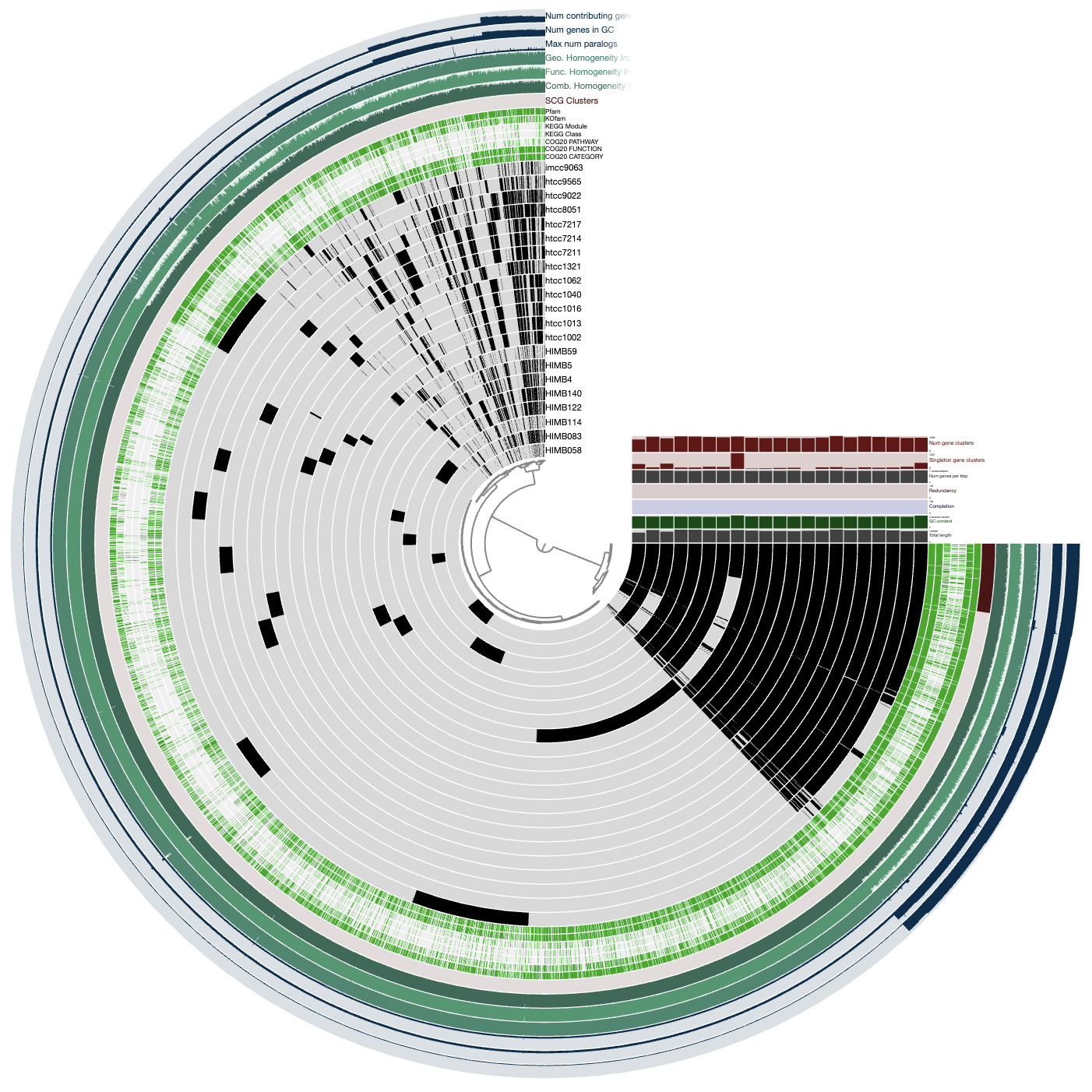
However, for the purposes of this study, we are done here. These pangenomes will be useful for some of the forthcoming analyses.