
Table of Contents
Microbiologists have been cultivating microbial organisms for centuries, and are now routinely using high-throughput sequencing technologies to access the genomic content of their culture collections, greatly enhancing our understanding of the microbial world.
In the best scenario, the investigated culture is axenic (i.e., entirely free of all other contaminating organisms) and no contamination has taken place during the extraction, purification, handling, and sequencing of the DNA. But unfortunately, non-axenic cultures, cross-contaminations, and even reagents regularly lead to the contamination of sequencing data being assembled for genomic recovery. Here is an incomplete, yet useful list of studies that discuss contamination sources:
- When Is a Microbial Culture “Pure”?
- Controlling for contamination in re-sequencing studies
- Microbiome science threatened by contamination
- Large-scale contamination of microbial isolate genomes by Illumina PhiX control
Accessing genomic contamination levels is important, but not enough
Great tools have been developed to estimate the level of completion of a given bacterial and archaeal draft genome, and perhaps more importantly, their level of contamination. For example, a recently published software dedicated to this task is CheckM. Briefly, these tools screen for marker genes that should be detected a very specific number of time in a given genome (often only one time). The less these gene markers are detected, the lower the completion. Inversely, the more they are detected above their theorical level, the more the contamination level will become. This is a very simple mathematical scheme based on our knowledge of bacterial and archaeal genomes and does not rely on any reference genome, which is particularly useful for environmental isolates. Keep in mind that such approach is generally reliable, but not perfect. This blog-post by Connor Skennerton describe some key pitfalls.
In general, it is important to access completion and contamination levels before going deeper into phylogeny, taxonomy and/or functionality of newly recovered genomes. This is obviously a critical moment for microbiologist who put all that effort into growing their culture (or into acquiring their single-cell genome). Optimally, your genome completion and contamination levels will verge around 100% and 0%, respectively. Note that a perfect 100% / 0% score is quite unlikely due to the imperfections of the approaches we rely on, however, a completion level of 90+% with <10% contamination is to be expected for a well-covered (i.e., deeply sequenced), and uncontaminated genome.
Unfortunately, your genome can be contaminated for multiple reasons. In general, the next step after detecting a problem is to fix it, right? But how fast, or how straightforward will it be to tease apart the genome of interest from the contamination? Eventually, you will realize that although they are very useful to estimate the level of contamination and completion, tools such as CheckM do not necessarily provide easy-to-use interfaces to manipulate, edit, and/or curate sreened genomes. This requires much more that simply screening for genes markers, and a platform dedicated to the processing and visualization of genomes using contextual information may be very helpful to explore your assembly, screen for unwanted contigs, and refine your genomes…
Well, not to brag about it, but this is exactly what anvi’o is designed for!
Using anvi’o to screen for possible contaminants and to curate individual genomes
You might have heard of anvi’o with respect to metagenomic binning, however, the platform is perfectly fit for enhanced genome-scale scrutiny and editing. Anvi’o checks for completion and contamination levels using four independently published single copy gene marker collections. But more importantly, anvi’o offers a fully equipped interface to detect and remove contaminants using relevant contextual information. Briefly, a tree is generated that displays contigs clustered based on their tetranucleotide frequencies (other clustering algorithms are available but might be more relevant to metagenomic assemblies). Multiple sources of information are subsequently displayed as layers around the tree and can be manipulated to access the biological relevance of any investigated “genome”.
In the case of uncontaminated genomes, the GC-content, coverage value, nucleotide variation density and (if available) taxonomical inference of each contigs should be somewhat similar across contigs. If not, it is generally easy to determine the contaminant fraction of the assembly (often one or multiple contig clusters that behave differently from the rest of the genome) and remove it from the genome selection. The user can simply select/unselect contigs and anvi’o automatically regenerates completion and contamination levels in a couple of second. It is therefore possible to test multiple contig selection configurations from the work environment before summarizing the “final” refined genome.
In this post I will describe two examples of assembled genomes from lab cultures processed with anvi’o: (I) an axenic, uncontaminated genome, (II) and a non axenic culture harboring multiple dominant populations, where the population of interest is the least abundant.
Example 1: axenic, uncontaminated culture
Here, I have an assembly ouput from an axenic, uncontaminated Bacteroides fragilis culture. This genome was sequenced on a HiSeq platfrom and a total of 33 contigs > 1kbp were generated, which totalled around 5 Mbp. I have processed the FASTA file of 33 contigs along with the BAM file of mapped short reads using anvi’o by (1) creating an contigs database using a split size of 2,000 nts (-L 2000), (2) running HMM profiles for single-copy genes, and (3) profiling the BAM file with an additional --cluster-contigs parameter (see the user tutorial for details of each step).
Once the profiling was complete, I started the interactive interface by typing:
anvi-interactive -p Example1/PROFILE.db -c contigs.db
If you are familiar with anvi’o you know that the interactive interface will start following this command. The most left panel in the figure below shows the initial, unedited tree of contigs in “mean coverage” view:
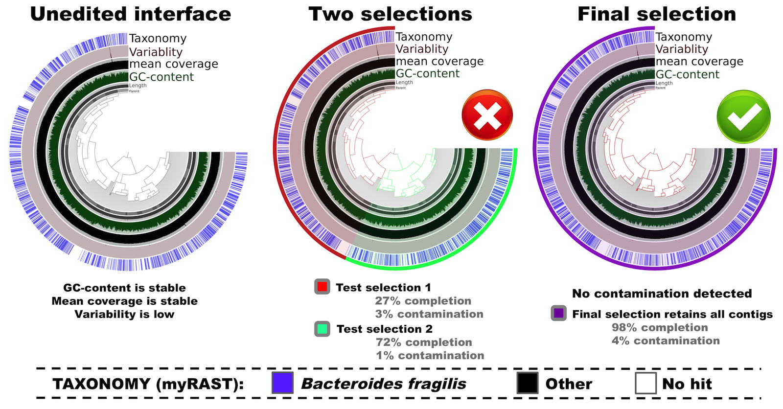
Here in this tree contigs are clustered based on their sequence composition (tetranucleotide frequency) alone.
In this example you can see all relevant metrics (i.e., mean coverage, GC-content, and taxonomical inference) are uniform across contigs. Furthermore, there is almost no variability, meaning that the variation density across the genome (number of positions with variable nucleoides per kilo base) is very low. This tells us that the cultivar is (mostly) clonal.
Let’s play a bit with the tree. There are two major clusters. First, I naively select the two apparent clusters into two different bins (see the center panel in the figure above). When I click on the tree to select these clusters, completion and contamination estimates are automatically calculated and displayed in the interface. In this scenario, selections have low contamination, as well as low completion levels. This doesn’t look optimal. But when I instead select all splits (see the right panel in the figure above), the completion estimate is now updated to 98%, while the contamination remains very low (<5%) –which is clearly much better than the “two clusters” scenario.
So this is my final selection for this genome, which is now ready to be summarized, and decorated with additional metadata (i.e., taxonomy, GC-content, functions, variability, etc).
Yet, one particular location of the genome looks intriguing… Do you see it too? Yes, I am talking about the bump in both the mean coverage, and the variability layers around the top of the trees in the figure above:
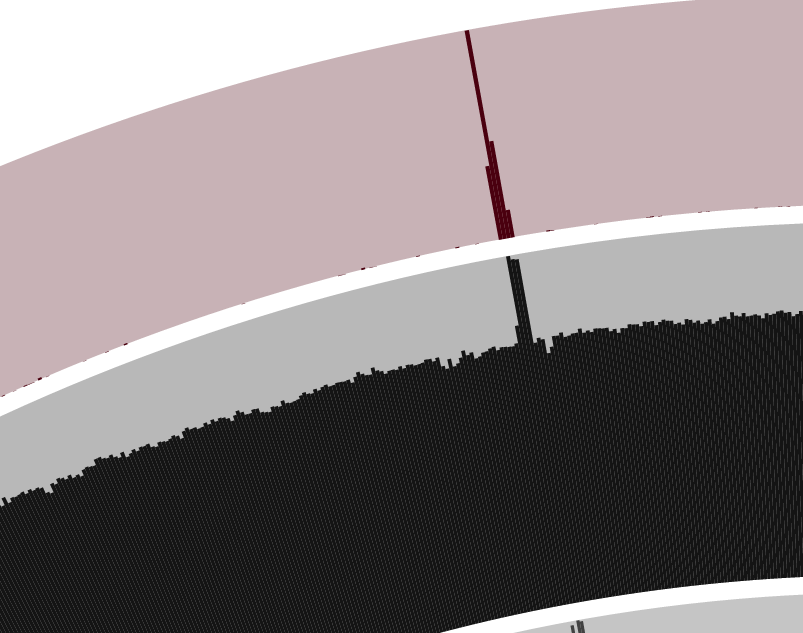
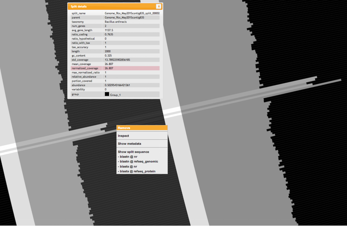
In general, when anvi’o detects variability and a stable coverage (compared to the rest of the genome), the variability is usually due to the natural polymorphism in a population. In metagenomic datasets we employ this information in an attempt to recover subtle, otherwise-missed ecological patterns. On the other hand, bumps in both variability and coverage suggest nothing but bad assembly of duplicate genes from a single “genotype”. Fortunately we can inspect these contigs to get a more detailed understanding using the interactive interface (by simply right-clicking on a split).
Let’s take a look at the variable, high-coverage region more closely. It is covered by 4 splits originating from the contig number 8. Splits are number 107, 108, 109 and 110. Here is what inspecting this region shows (the figure below shows multiple splits as I simply put multiple inspection screenshots in one page for brevity):
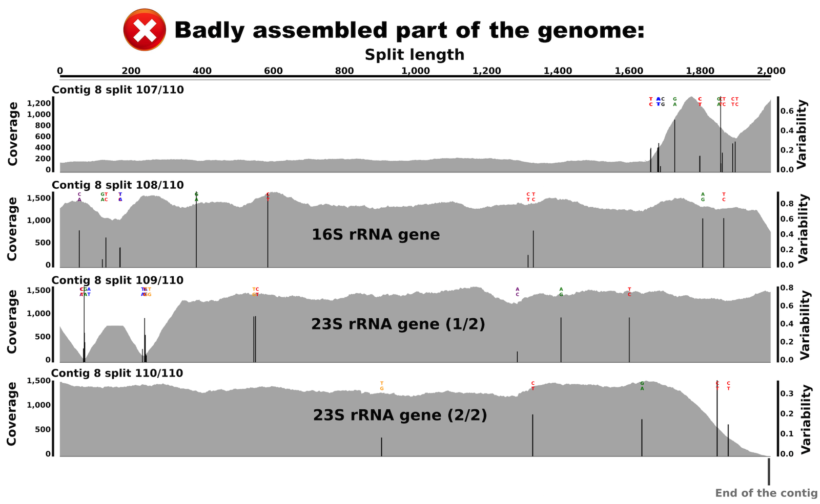
We can see that coverage is stable in both splits, but with a difference of about 6 fold compared to the rest of the genome. Interestingly, we can also see various nucleic acid positions with nucleotide variation in these splits. This explains the bump in the variability layer from the interface view.
When I BLAST searched these splits, I recovered that split 108 harbors most of the 16S rRNA gene, while splits 109 and 110 harbor the 23S rRNA gene! So, we learn two things from this: (I) there is about 6 copies of the 16S-23S rRNA operon in this genome that were misassembled into a single contig, (II) and these copies are not identical as indicated by multiple nucleotide variation positions in both the 16S rRNA gene and the 23S rRNA gene.
This is not a contamination, but an assembly issue, which anvi’o cannot fix. The concept of decreasing entropy while increasing the biological relevance of sequences has already been successfully applied to 16S rRNA gene amplicons (see Oligotyping and Minimum Entropy Decomposition, but as of today we are missing a comparable approach for genomics and metagenomics.
Example 2: non-axenic culture of 3 distinct bacterial populations
For the second example I obtained an assembly from a non axenic bacterial culture. The sample was sequenced on a HiSeq platfrom, and a total of 3,278 contigs > 1kbp were generated, representing around 11.5 Mbp. At this point we already knew something was probably wrong because most bacterial genomes have a length of 1-9 Mbp. To learn more about this assembly, we processed the 3,278 contigs along with the BAM file of mapped reads in anvi’o, using the exact same parameters as for the first example. The 3,278 contigs were fragmented into 6,063 splits.
Here is the summary of hits for each single copy gene collection:
- HMM Profiling for Alneberg et al (34 single copy genes): 86 hits
- HMM Profiling for Dupont et al (111 single copy genes): 248 hits
- HMM Profiling for Creevey et al (40 single copy genes): 115 hits
Even from the initial HMM results it is clear that this is quite a mixed sample (and it is also clear that there are about three genomes in it).
The following figure is what shows up after running the interactive interface, and editing the tree by selecing the 3 main clusters (left panel):
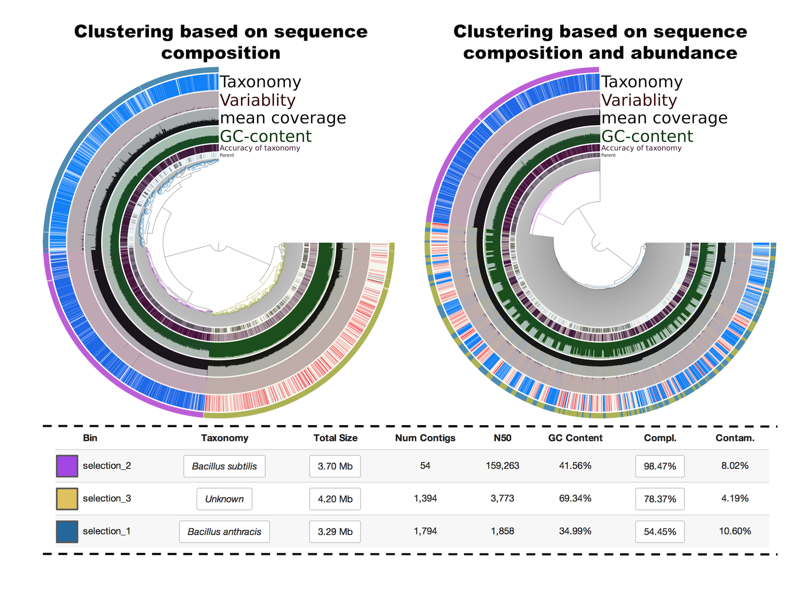
Selections 1 and 2 have the same taxonomical inference and GC-content but a very distinct mean coverage (around 10X versus around 120X). Because the clustering is based on sequence composition, we also know that they have distinct tetranucleotide frequencies. Finally, the selection 3 has a different taxonomical inference (in this particular case this was the originally targeted genome), a much higher GC-content, and a mean coverage similar to contigs from the selection 1. For curiosity, I also visualized the tree based on a different clustering that takes also into account coverage values (right panel). This feature is very useful for metagenomic binning when multiple samples are analysed. But here, with a single sample, the clustering simply mixes selections 1 and 3, which is not very useful for binning or fixing contaminations. So in this example, we started with a highly contaminated assembly to identifying 3 draft genomes that display medium to high completion and low contamination levels.
Sequence composition is very useful but some manual editing was required in this example, especially for the two first selections that represent closely related organisms. Here is an example of how easy it is to look for inconsistent coverage across splits and remove them from a bin with a simple right-click (the two layers in the figure are normalized coverage and mean coverage):
Concluding remarks
Scrutinizing genomes using FASTA files and associated mapped reads (raw sequences or BAM files) is a straightforward proccess with anvi’o. Such efforts may improve removing contaminants from genomic projects, and refine the tree of life. contigs