Table of Contents
We have a citable version, and a more formal description of this workflow in our recent paper “Identifying contamination with advanced visualization and analysis practices: metagenomic approaches for eukaryotic genome assemblies” (see the supplementary material).
Your ability to identify genomes appropriately from an assembly will depend on many factors, such as the number of samples you have to exploit the differential coverage patterns of genomes, or the algorithm you use to tease apart that information. But even before doing any of the real binning, you may have a rough answer to this question by just taking a quick look from your contigs:
How many bacterial genomes should I expect to find in these contigs I assembled from my shotgun data?
Anvi’o has been very practical for us to answer this, and here you will find the workflow to try it on your own FASTA file of contigs.
The workflow
PLEASE USE anvi-display-contigs-stats for this task. The rest of the post is here for historical reasons, but basically this functionality is now implemented in this program.
I will describe the three anvi’o steps using Sharon et al.’s infant gut study as an example. The contigs.fa file I will use is this section is the co-assembly of all samples in Sharon et al’s study.
As a reminder, Sharon et al. identified 12 bacterial draft genomes in this dataset, 8 of which were complete or near-complete. Our re-analysis of this dataset in the anvi’o methods paper also yielded similar resulted (you can find more about our re-analysis here).
Generating a contigs database
First, you will need to introduce anvi’o to your contigs by generating a contigs database –one of the essential files of the anvi’o workflow.
$ anvi-gen-contigs-database -f contigs.fa -o contigs.db -n 'My contigs db'
And this is how this goes on my screen:
$ anvi-gen-contigs-database -f contigs.fa -o contigs.db -n 'My contigs db'
Contigs database .............................: A new database, new-contigs.db, has been created.
Number of contigs ............................: 4,189
Number of splits .............................: 4,861
Total number of nucleotides ..................: 35,766,167
Split length .................................: 20,000

Finding ORFs in contigs
===============================================
Genes ........................................: /var/folders/nm/jmps9l7j7w1dr8rbpv119zgr0000gn/T/tmpZN2Fwt/contigs.genes
Proteins .....................................: /var/folders/nm/jmps9l7j7w1dr8rbpv119zgr0000gn/T/tmpZN2Fwt/contigs.proteins
Log file .....................................: /var/folders/nm/jmps9l7j7w1dr8rbpv119zgr0000gn/T/tmpZN2Fwt/00_log.txt
Result .......................................: Prodigal (v2.6.2) has identified 32265 genes.

Contigs with at least one gene call ..........: 4174 of 4189 (99.6%)
Looking for single-copy genes
Now we have the contigs database, the next thing we will do is to look for bacterial single copy genes. If you have read our article you already know that anvi’o installs with four single-copy gene collections from four different groups.
All you need to do is to run this command for HMM hits for thoese gene collections to be added to the database you just created:
$ anvi-run-hmms -c contigs.db
And this is how this step goes on my screen as anvi’o goes through each single-copy gene collection:
$ anvi-run-hmms -c contigs.db
HMM profiles .................................: 4 sources have been loaded: Alneberg_et_al (34 genes), Dupont_et_al (111 genes), Campbell_et_al (139 genes), Creevey_et_al (40 genes)
Sequences ....................................: 32265 sequences reported.
FASTA ........................................: /var/folders/nm/jmps9l7j7w1dr8rbpv119zgr0000gn/T/tmpU2EHjX/sequences.fa

HMM Profiling for Alneberg_et_al
===============================================
Reference ....................................: Alneberg et al, http://www.nature.com/nmeth/journal/v11/n11/full/nmeth.3103.html
Pfam model ...................................: /Users/meren/Desktop/MBL/anvio/anvio/data/hmm/Alneberg_et_al/genes.hmm.gz
Number of genes ..............................: 34
Temporary work dir ...........................: /var/folders/nm/jmps9l7j7w1dr8rbpv119zgr0000gn/T/tmpq6RiH1
HMM scan output ..............................: /var/folders/nm/jmps9l7j7w1dr8rbpv119zgr0000gn/T/tmpq6RiH1/hmm.output
HMM scan hits ................................: /var/folders/nm/jmps9l7j7w1dr8rbpv119zgr0000gn/T/tmpq6RiH1/hmm.hits
Log file .....................................: /var/folders/nm/jmps9l7j7w1dr8rbpv119zgr0000gn/T/tmpq6RiH1/00_log.txt
Number of raw hits ...........................: 368

HMM Profiling for Dupont_et_al
===============================================
Reference ....................................: Dupont et al, http://www.nature.com/ismej/journal/v6/n6/full/ismej2011189a.html
Pfam model ...................................: /Users/meren/Desktop/MBL/anvio/anvio/data/hmm/Dupont_et_al/genes.hmm.gz
Number of genes ..............................: 111
Temporary work dir ...........................: /var/folders/nm/jmps9l7j7w1dr8rbpv119zgr0000gn/T/tmpRPCMEL
HMM scan output ..............................: /var/folders/nm/jmps9l7j7w1dr8rbpv119zgr0000gn/T/tmpRPCMEL/hmm.output
HMM scan hits ................................: /var/folders/nm/jmps9l7j7w1dr8rbpv119zgr0000gn/T/tmpRPCMEL/hmm.hits
Log file .....................................: /var/folders/nm/jmps9l7j7w1dr8rbpv119zgr0000gn/T/tmpRPCMEL/00_log.txt
Number of raw hits ...........................: 886

HMM Profiling for Campbell_et_al
===============================================
Reference ....................................: Campbell et al, http://www.pnas.org/content/110/14/5540.short
Pfam model ...................................: /Users/meren/Desktop/MBL/anvio/anvio/data/hmm/Campbell_et_al/genes.hmm.gz
Number of genes ..............................: 139
Temporary work dir ...........................: /var/folders/nm/jmps9l7j7w1dr8rbpv119zgr0000gn/T/tmp9XgXUp
HMM scan output ..............................: /var/folders/nm/jmps9l7j7w1dr8rbpv119zgr0000gn/T/tmp9XgXUp/hmm.output
HMM scan hits ................................: /var/folders/nm/jmps9l7j7w1dr8rbpv119zgr0000gn/T/tmp9XgXUp/hmm.hits
Log file .....................................: /var/folders/nm/jmps9l7j7w1dr8rbpv119zgr0000gn/T/tmp9XgXUp/00_log.txt
Number of raw hits ...........................: 1,361

HMM Profiling for Creevey_et_al
===============================================
Reference ....................................: Creevey et al, http://journals.plos.org/plosone/article?id=10.1371/journal.pone.0022099
Pfam model ...................................: /Users/meren/Desktop/MBL/anvio/anvio/data/hmm/Creevey_et_al/genes.hmm.gz
Number of genes ..............................: 40
Temporary work dir ...........................: /var/folders/nm/jmps9l7j7w1dr8rbpv119zgr0000gn/T/tmp2GoYlD
HMM scan output ..............................: /var/folders/nm/jmps9l7j7w1dr8rbpv119zgr0000gn/T/tmp2GoYlD/hmm.output
HMM scan hits ................................: /var/folders/nm/jmps9l7j7w1dr8rbpv119zgr0000gn/T/tmp2GoYlD/hmm.hits
Log file .....................................: /var/folders/nm/jmps9l7j7w1dr8rbpv119zgr0000gn/T/tmp2GoYlD/00_log.txt
Number of raw hits ...........................: 432
So far so good.
Visualizing the results
Now we have a contigs database with everything we need. It is time to visualize the results. For now this is a two-step process. First we need to generate essential input files for the R program that will do the visualization:
$ anvi-script-gen_stats_for_single_copy_genes.py contigs.db
This should generate two new files in the directory:
$ ls
contigs.db  contigs.db.genes  contigs.db.genes
And the final step is to visualize the information reported in those files:
$ anvi-script-gen_stats_for_single_copy_genes.R contigs.db.hits contigs.db.genes
[1] "Alneberg_et_al"
[1] "Creevey_et_al"
[1] "Campbell_et_al"
[1] "Dupont_et_al"
Which should generate a PDF file in the same directory if you have a proper R installation:
$ ls
contigs.db  contigs.db.genes  contigs.db.genes  contigs.db.hits_e_1_new.pdf
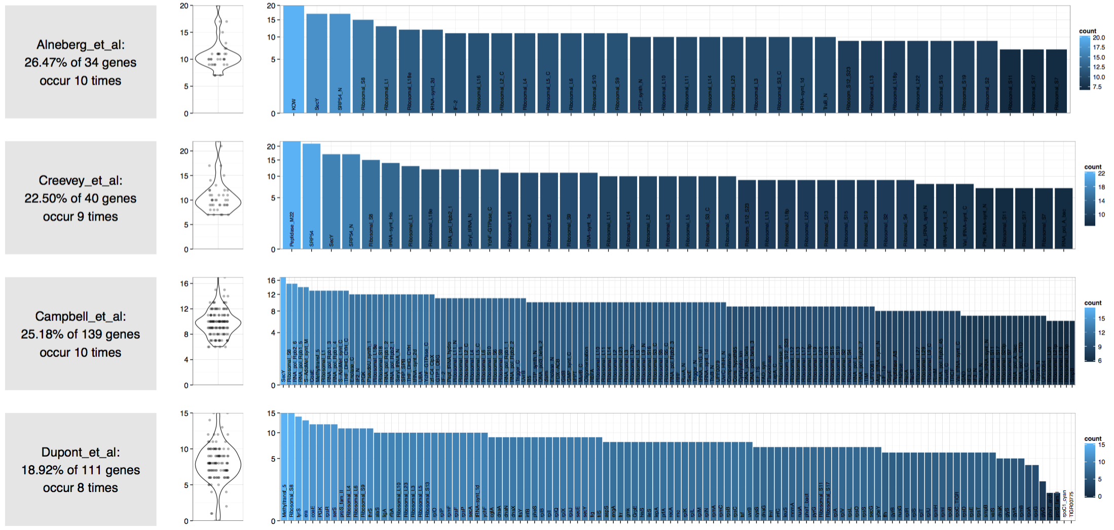
Here is the result:
Which suggests that there are 8 to 10 genomes in this assembly!
Other examples
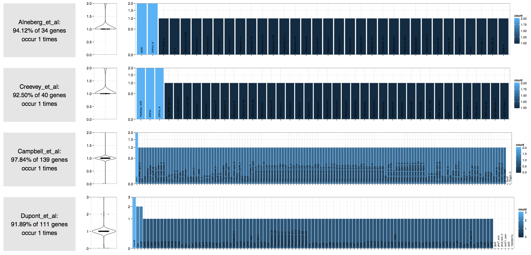
Here is the result of the worfklow I described above on an assembly generated from the shotgun seqeuncing of a cultivar:
| Source | Number of expected bacterial genomes |
|---|---|
| Alneberg et al. | 1 |
| Creevey et al. | 1 |
| Campbell et al. | 1 |
| Dupont et al. | 1 |
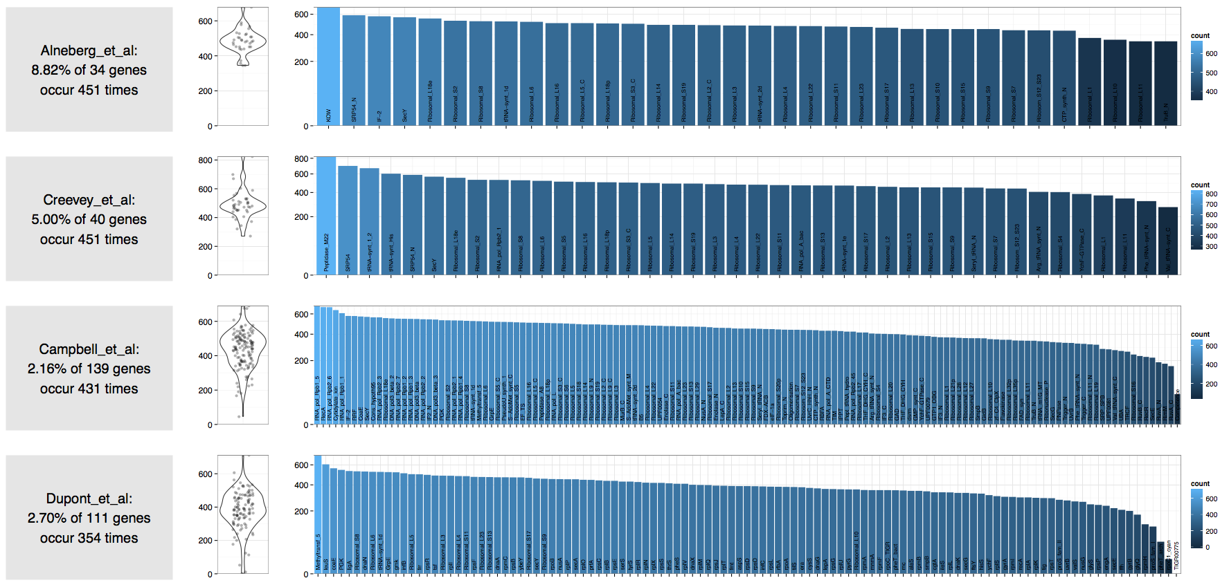
In contrast an ocean sample we assembled recently:
| Source | Number of expected bacterial genomes |
|---|---|
| Alneberg et al. | 451 |
| Creevey et al. | 451 |
| Campbell et al. | 431 |
| Dupont et al. | 354 |
Clearly these estimations are mere approximations at best, and should be taken with a grain of salt. However, they do give a rough idea about the complexity of a given metagenome, and what you should expect to get from it.
Please don’t hesitate to use the comments section for your suggestions, and please keep an eye on our repository.


