
Table of Contents
Mike’s preface
If you have been using anvi’o’s interactive interface without an anvi’o expert sitting right next to you, then you probably have found yourself at some point wondering whether these ‘views’ you were exploring actually meant what you thought they did.
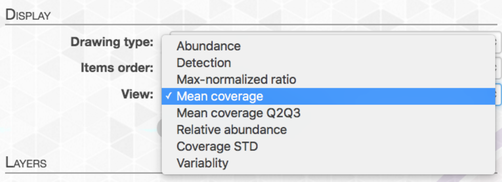
Sure there are some pretty safe ones that you can rationalize to yourself with some confidence, like “Mean coverage”, or “Mean coverage Q2Q3”, for example. But even those that seem relatively straightforward, like “Relative abundance”, can be pretty tricky. Relative to what? All samples? All contigs? And don’t even get me started on “Detection”! (Meren’s taken quite a bit of heat for this term’s ambiguity, and rightfully so, hehe).
I’ve certainly sent my fair share of emails to the team asking to clarify a view I thought I had pinned down, and in some cases it turned out I was slightly (or completely) wrong. So the last time I was in the same city as Meren, I made sure he went over these with me, several times, in painstakingly repetitive detail for him I’m sure :). But I convinced him it was worth his time to do so by saying I’d make a blog post about it to hopefully help others too.
So first here’s a quick reference table, and after that I’ll try to highlight some of the nuances in more detail and give examples where each can be particularly useful.
For contigs larger than a certain size (20,000 bp by default), anvi’o splits these into smaller fragments it aptly identifies as ‘splits’ – for reasons discussed in the original paper. Technically, all of the interactive ‘views’ act on the ‘split’ level if a contig was split, and the contig level if it wasn’t split. For simplicity’s sake within this document, you will see ‘contig’, but that’s referring to whatever the leaf you are looking at happens to be.
| View | Value |
|---|---|
| Abundance | mean coverage of a contig divided by overall sample mean coverage |
| Relative abundance | # of reads recruited to a contig divided by total reads recruited to that contig across all samples |
| Max-normalized ratio | # of reads recruited to a contig divided by the maximum number of reads recruited to that contig in any sample |
| Mean coverage | average depth of coverage across contig |
| Mean coverage Q2Q3 | average depth of coverage excluding nucleotide positions with coverages in the 1st and 4th quartiles |
| Detection | proportion of nucleotides in a contig that are covered at least 1X |
| Coverage STD | standard deviation of coverage for a given contig |
| Variability | SNVs per kbp |
For those above that are provided as a summary for a bin or MAG, they consider all of the contigs of that bin/MAG as though they were one. For example, “Detection” of an entire bin would be the proportion of all of the bases of that bin that are covered at least 1X. It is not an average of all of the individual contigs’ detections.
Anvi’o views
Mean coverage
Average depth of coverage across contig.
Add up the coverage of each nucleotide in a contig, and divide by the length of the contig. This is the default view in most cases.
Mean overage Q2Q3
Average depth of coverage across contig excluding nucleotide positions with coverage values falling outside of the interquartile range for that contig.
Calculated the same as mean coverage, except only incorporating those nucleotide coverage values that fall within 2nd and 3rd quartiles of the distribution of nucleotide coverages for that contig. This can help smooth out the mean coverage visualization by removing nucleotide coverage values from the equation that may be outliers due to non-specific mapping.
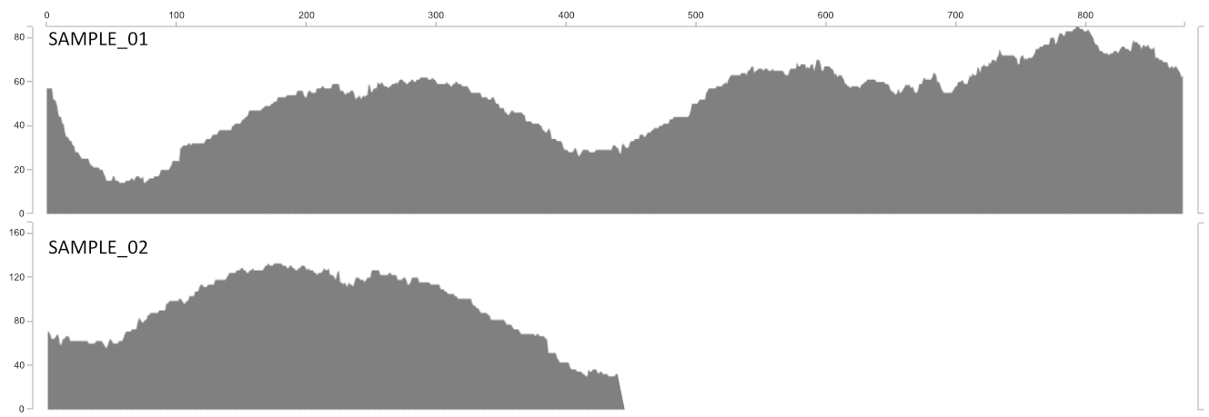
Detection
The proportion of a given contig that is covered at least 1X.
Detection gives you an idea of how much of the contig actually recruited reads to it. The utility of this is most clearly demonstrated with the following figure. Sample_1 and Sample_2 may have the same mean coverage (say ~50x). However, Sample_1’s detection would be 1.0 (as all nucleotides in the contig are covered by at least one read), while Sample_2’s detection would be ~0.5. From the main interactive interface, mean coverage would appear to be consistent between these contigs. But the detection view would show you at a glance that something funny is going on that probably needs a closer look.
Abundance
Mean coverage of a contig divided by that sample’s overall mean coverage.
Abundance for a contig is constrained to within one sample. In a sense this view is telling you that those contigs with larger abundance values are more represented in that sample (i.e. recruited more reads) than those contigs with smaller abundance values. And it does this by providing the ratio of that contig’s mean coverage to that sample’s overall mean coverage incorporating all contigs. So if your abundance value is 2, that contig’s mean coverage is twice that of the mean for all contigs in that sample.
Relative abundance
Proportion of reads recruited to a contig out of the total reads recruited to that contig across all samples.
Relative abundance considers one contig across all samples. This will tell you in which sample a particular contig recruited the most reads. Since it is normalized to the total number of reads recruited to contig across all samples, values from all samples for a given contig will always sum to 1.
Max-normalized ratio
Proportion of reads recruited to a contig out of the maximum number of reads recruited to that contig in any sample.
This also considers one contig across all samples. But in this case the value is normalized to the single maximum value for that contig (as opposed to the sum as in relative abundance). Because of this the sample containing the contig that contributed the max value will always equal 1, and the value for that contig in the other samples will be the fraction of that max.
Coverage STD
The standard deviation of coverage values for a given contig.
This is constrained to an individual contig in an individual sample, and represents the standard deviation of the nucleotide coverage values in that contig.
Variability
Number of reported single-nucleotide variants per kilo base pair.
This gives you a view of SNV density of each contig. This can give you an idea of how much variability there is in the reads that successfully recruit to that contig. If resolving closely related populations of organisms is something you’re interested in, be sure to check out this and this.
The capabilities of anvi’o are constantly expanding, but the heart of the interactive interface lies with facilitating the manual curation of metagenomic bins. All of these views utilizing different metrics are here to help in that effort of identifying which contigs (or splits) likely originate from a similar source. It’s certainly a good idea to take a peek at multiple views when refining your bins, so be sure to take advantage of them!