A simple read recruitment exercise

Downloading the data pack
Preparation
Read recruitment
Recruiting reads from multiple samples in a loop
Taking a look at the read recruitment results

Does every individual carry a microbial population that matches this genome?
Does every gene in this genome occur in every individual?

Real-world examples

Summary

The purpose of this mini exercise is to walk you through a simple read recruitment experiment. Throughout this exercise you will use a mock dataset to,

Familiarize yourself with commonly used file formats such as FASTA, FASTQ, SAM, and BAM,
Learn the basic steps of read recruitment through Bowtie2 and samtools,
Learn how to profile read recruitment results using anvi’o,
Familiarize yourself with downstream steps of the analysis of recruited reads.

If you have any questions about this exercise, or have ideas to make it better, please feel free to get in touch with the anvi’o community through our Discord server:

Questions? Concerns? Find us on

To follow this exercise, you should first follow the instructions here that will install anvi’o on your computer along with its dependencies.

This exercise uses a mock dataset we have generated for you that includes a reference sequence and some short reads to mimic a common scenario in read recruitment analyses.

The main purpose of a typical read recruitment analysis is to investigate one or more reference sequences in the context of one or more samples to which we have access thorugh short reads. Your references and short reads can be anything.

The set of reference sequences, which often is described as a FASTA file, can be one or more contiguous segments of DNA (contigs) that may belong to a single genome. Or you may put together a bunch of genomes in a single FASTA file. Your reference seqeunces may be describing genes, partial or entire metagenome-assembled genomes, single-amplified genomes, isolate genomes, viral genomes, or plasmids. Any sequence that is longer than your short reads may serve a reference.
The set of short reads can also be a lot of things. They may be coming from the sequencing of a single genome, an entire metagenome, or even amplicons generated using primers. They don’t even need to be short, in fact. You can recruit long-reads with your reference sequences, too.

Essentially, you have a lot of freedom to define your reference sequence context and short reads depending on the question you wish to answer. But one thing is certain: when used right, read recruitment can answer many questions in microbiology.

For the sake of simplicity, here we will start with a boring example: a single genome and a set of mock metagenomes, since the purpose of this tutorial is to offer you some hands-on exposure to read recruitment rather than science it enables.

Let’s start.

Downloading the data pack

First, open your terminal, go to any directory you like, and download the data pack we have stored online for you:

curl -L https://figshare.com/ndownloader/files/31180186 \
     -o metagenomic-read-recruitment-data-pack.tar.gz

Then unpack it, and go into the data pack directory:

tar -zxvf metagenomic-read-recruitment-data-pack.tar.gz

cd metagenomic-read-recruitment-data-pack

At this point, if you type ls in your terminal, this is what you should be seeing:

genomes.fa metagenomes/

The file genome.fa is our reference sequence (which happens to be a microbial genome with only one contig, and the directory metagenomes includes multiple mock metagenomes.

Throughout this exercise we will assume that these are human gut metagenomes.

Preparation

Since we are going to be using anvi’o to characterize the read recruitment results, the first step is to do something that has nothing to do with read recruitment, but necessary for downstream anvi’o analyses: turning our genome into a contigs-db. Which is a simple step that uses the program anvi-gen-contigs-database:

anvi-gen-contigs-database -f genome.fa \
                          -o genome.db

The online documentation on contigs databases suggest running the following optional programs on any contigs database to annotate its genes with functions, identify single-copy core genes in it, and enrich it with taxonomic information. While we are here, let’s run those programs on our genome as well.

anvi-run-ncbi-cogs -c genome.db --num-threads 4

anvi-run-hmms -c genome.db

anvi-run-scg-taxonomy -c genome.db --num-threads 4

Now we are done with the anvi’o side of things for now.

Read recruitment

There are many bioinformatics tools to map reads to a reference context. Here we will use Bowtie2. Like many high-performance tools for similar purpose, Botwie2 requires us to turn our genome sequence into a special file format that is much more computationally accessible. For this, we use the program bowtie2-build:

bowtie2-build genome.fa genome

If you look at your directory again, you will see the additional files this step has generated. Now we are ready for the actual read recruitment analysis.

To actually perform the read recruitment analysis for a single individual, one would need to (1) perform the read recruitment and store the results in a SAM file

bowtie2 -x genome \
        -1 metagenomes/magdalena-R1.fastq \
        -2 metagenomes/magdalena-R2.fastq \
        -S magdalena.sam

(2) convert the SAM file into a BAM file,

samtools view -F 4 \
              -bS magdalena.sam \
              -o magdalena-RAW.bam

(3) sort and index the BAM file:

samtools sort magdalena-RAW.bam -o magdalena.bam
samtools index magdalena.bam

At this stage you are literally done with read recruitment, and all the information is stored in the BAM file that is accessible to other programs for downstream analyses.

Anvi’o is one of those programs that can make sense of BAM files. Using the anvi’o program anvi-profile, we can ‘profile’ the contents of a given BAM file:

anvi-profile -i magdalena.bam \
             -c genome.db \
             -o magdalena-profile \
             --cluster

The --cluster parameter is optional, and only is necessary for anvi’o to add necessary information for itself to be able to visualize single profiles.

The program anvi-profile processes the raw data stored in a BAM file and turns it into a more accessible format, which is called profile-db in the anvi’o universe. For instance, since we already have our profile database, we can see the read recruitment results for this single sample in the anvi’o interactive interface using the program anvi-interactive:

anvi-interactive -c genome.db \
                 -p magdalena-profile/PROFILE.db

We are done with one of the metagenomes. Four to go.

Recruiting reads from multiple samples in a loop

Running the lines above for each individual one by one would have generated all the profiles we would have needed to survey our genome across multiple individuals.

But to save time and minimize human error, we can create a ‘for loop’ in the shell to run these redundant steps for each individual.

Please note that the name magdalena is not included below since we already have generated a profile database for this person.

for person in batuhan alejandra jonas jessika
do
    echo "Working on ${person} ..."
    bowtie2 -x genome -1 metagenomes/${person}-R1.fastq -2 metagenomes/${person}-R2.fastq -S ${person}.sam
    samtools view -F 4 -bS ${person}.sam -o ${person}-RAW.bam
    samtools sort ${person}-RAW.bam -o ${person}.bam
    samtools index ${person}.bam
    anvi-profile -i ${person}.bam -c genome.db -o ${person}-profile
    rm -rf ${person}.sam ${person}-RAW.bam
done

Instead of copy-pasting the lines above, one can store them in a file (e.g., profile.sh), and run the contents of the file instead:

bash profile.sh

A successful completion of the these steps should result in five single profiles that look like this:

ls */PROFILE.db
alejandra-profile/PROFILE.db  batuhan-profile/PROFILE.db  jessika-profile/PROFILE.db  jonas-profile/PROFILE.db  magdalena-profile/PROFILE.db

Now we could use another anvi’o program, anvi-merge, to merge these individual profiles into a final merged profile database:

anvi-merge *-profile/PROFILE.db \
           -c genome.db \
           -o merged-profiles

Now we are ready to investigate things a bit deeper.

Taking a look at the read recruitment results

Following the data preparation steps I detailed in the previous section, we can start focusing on some individual questions.

Does every individual carry a microbial population that matches this genome?

To investigate the occurrence of this genome in metagenomes from the individuals in the data pack, we can visualize the merged profile of read recruitment results the way we did it for a single sample previously using the program anvi-interactive once again:

anvi-interactive -p merged-profiles/PROFILE.db \
                 -c genome.db

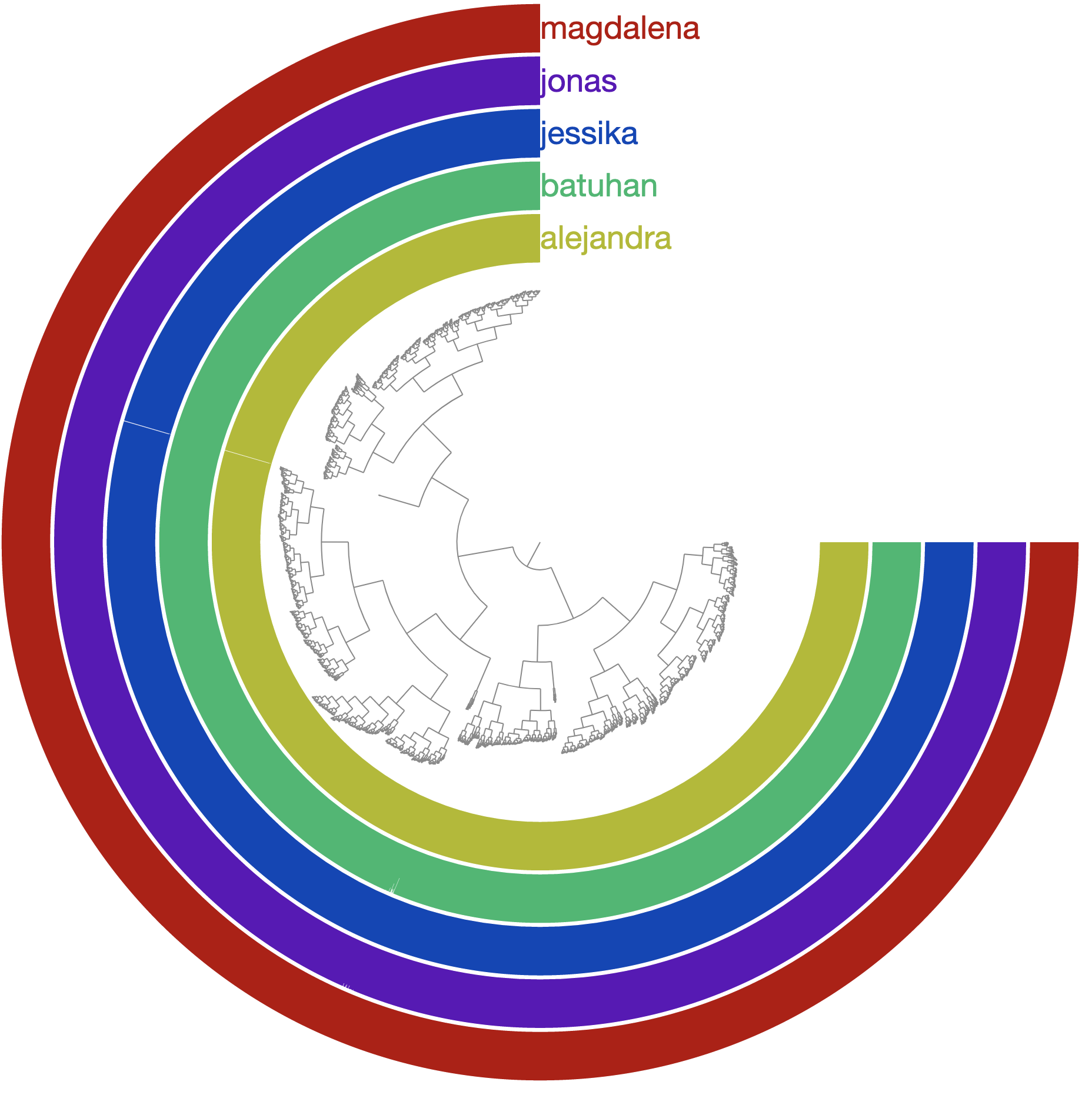
Which should give you the following display:

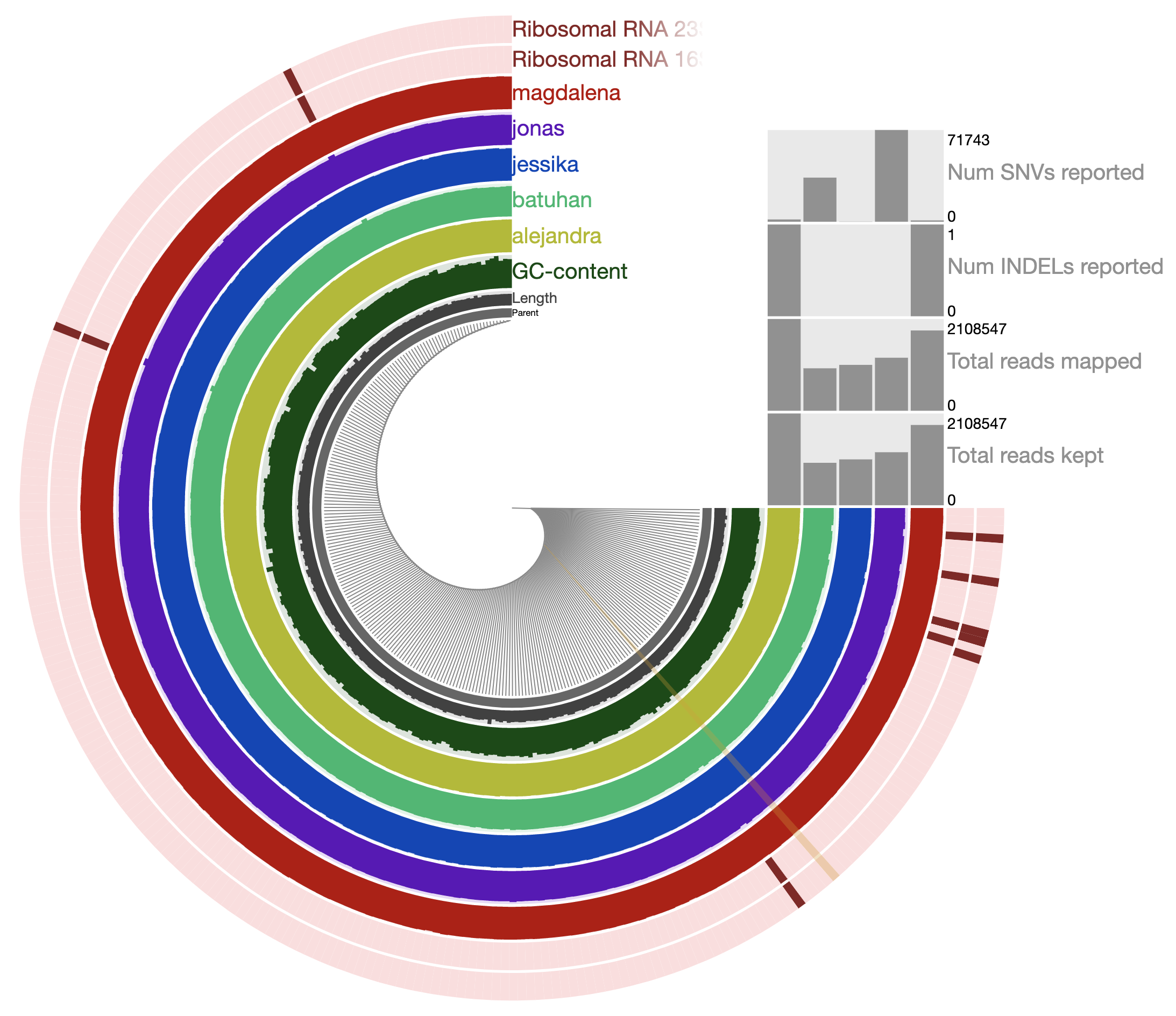
Every piece of this genome seems to be recruiting a lot of reads from every individual. In fact, inspecting the coverage of a random contig, one could see that the average coverage of the genome across these individuals is between about 20X to 40-50X:

So indeed, we happened to have a genome that very well represents a population in every individual.

Does every gene in this genome occur in every individual?

Since it was difficult to answer this question by visualizing mean coverage values at the ‘contig’ level, we can use the program anvi-interactive in a different mode: --gene-mode.

Although, according to the help menu of the program, this mode requires a collection of contigs to focus on. The utility of this requirement comes from the fact that if you are working with a large number of genomes, and if you wish to visualize gene-level coverage values of a single genome in your data set, you would have to tell anvi’o explicitly which set of contigs in your contigs-db belongs to which genome. Since we are in fact working with a single genome in this particular example, we simply need a collection that describes all contigs in our contigs-db in a single bin. Luckily, there is an anvi’o program for this boring task:

anvi-script-add-default-collection -p merged-profiles/PROFILE.db

Now we can ask anvi’o to visualize coverage values of each gene in the bin called ‘EVERYTHING’ the following way:

anvi-interactive -p merged-profiles/PROFILE.db \
                 -c genome.db \
                 -C DEFAULT \
                 -b EVERYTHING \
                 --gene-mode

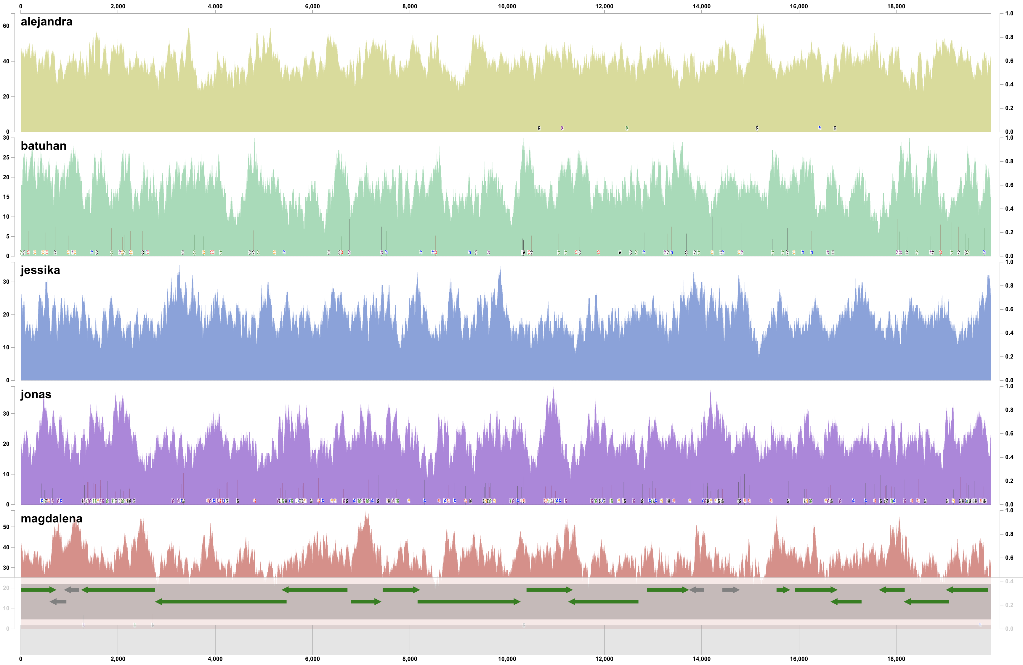
This should give you the gene-level coverages:

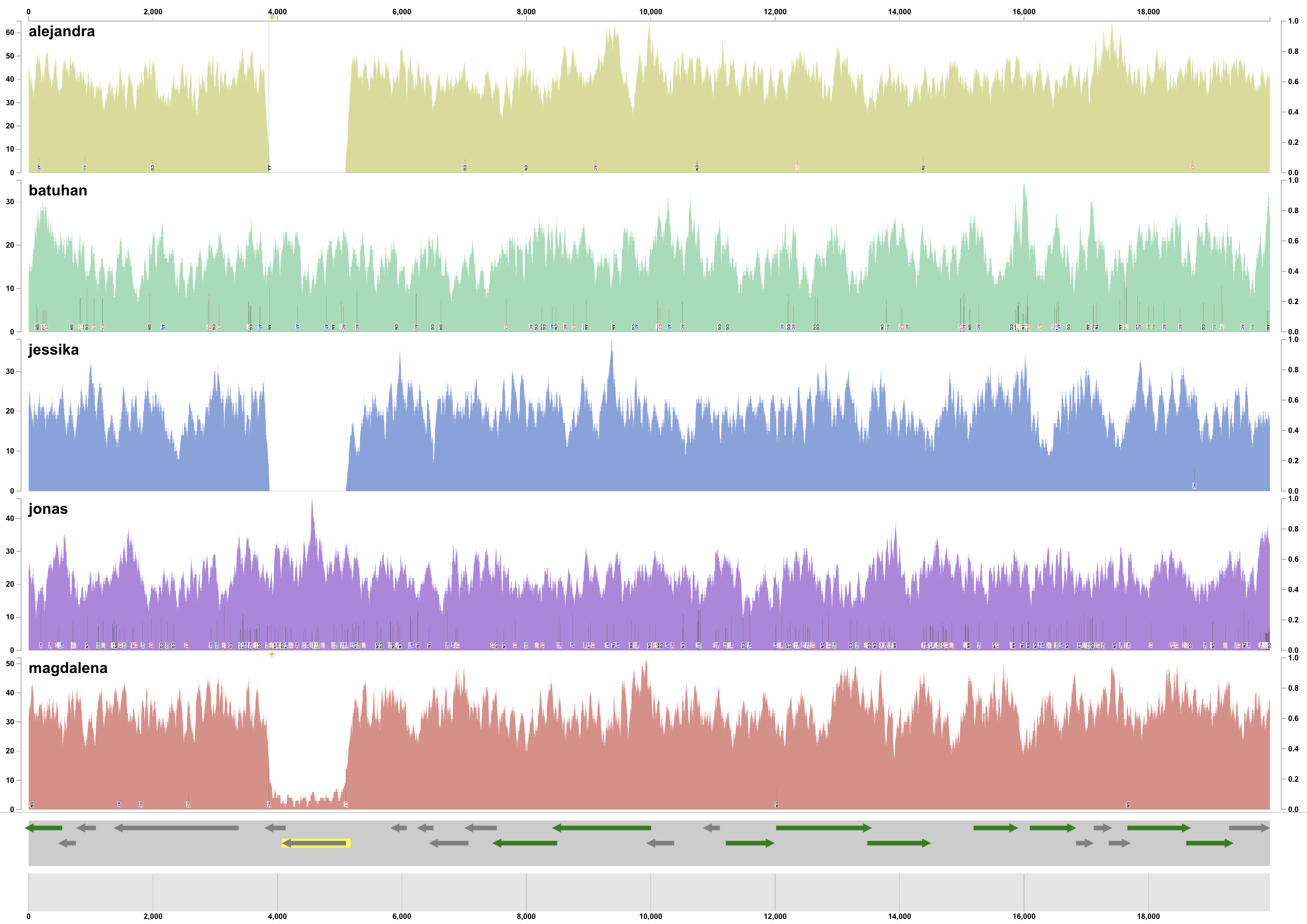
Even in this mock example, the coverage of genes varies across the genome. Which is expected even in real-world cases: the coverage of genes in a single genome will differ from one another in the same environment, and across environments. Another way to visualize covearge statistics is to focus on the detection value, which often can reveal things that are too subtle to be captured by mean coverage alone. We can easily switch to ‘detection’ view of our data through the interface, which should present us with this view:

Which immediately reveals multiple genes that were not detected in some of the metagenomes:

It turns out, not all genes in this genome are present in populations across different individuals.

The anvi’o inspection page is extremely useful to learn more about individual genes, their synteny, and coverages. One can make many observations by simply staring at these pages:

These genes happen to lack functional annotations, yet, clicking on them also presents us with an option to recover their sequences:

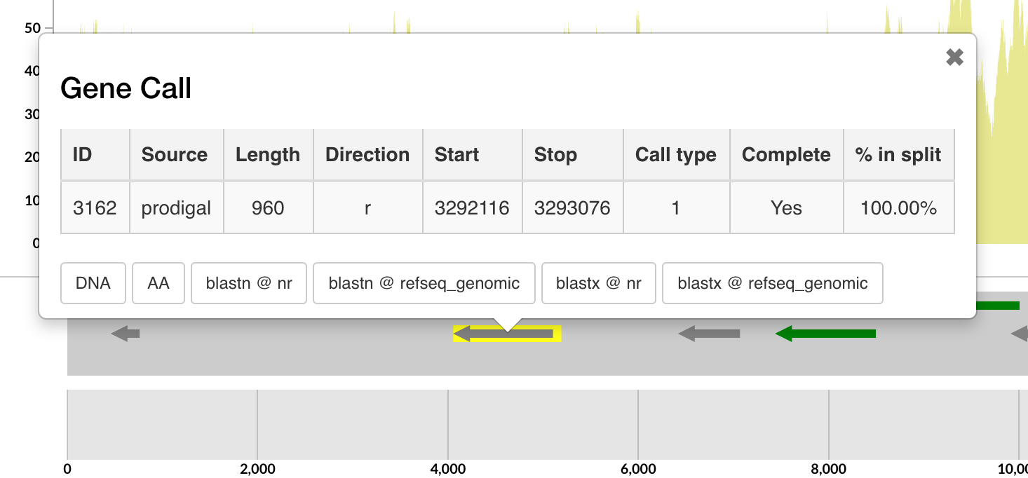
Here is the sequence of the short one:

>3161|contig:genome|start:3291835|stop:3292105|direction:r|rev_compd:True|length:270
MKKMFMAVLFALASVNAMAADCAKGKIEFSKYNEDDTFTVKVDGKEYWTSRWNLQPLLQSAQLTGMTVTIKSSTCESGSGFAEVQFNND

And the long one:

>3162|contig:genome|start:3292116|stop:3293076|direction:r|rev_compd:True|length:960
MKCILFKWVLCLLLGFSSVSYSREFTIDFSTQQSYVSSLNSIRTEISTPLEHISQGTTSVSVINHTPPGSYFAVDIRGLDVYQARFDHLRLIIEQNNLYVAGFVNTATNTFYRFSDFTHISVPGVTTVSMTTDSSYTTLQRVAALERSGMQISRHSLVSSYLALMEFSGNTMTRDASRAVLRFVTVTAEALRFRQIQREFRQALSETAPVYTMTPGDVDLTLNWGRISNVLPEYRGEDGVRVGRISFNNISAILGTVAVILNCHHQGARSVRAVNEESQPECQITGDRPVIKINNTLWESNTAAAFLNRKSQFLYTTGK

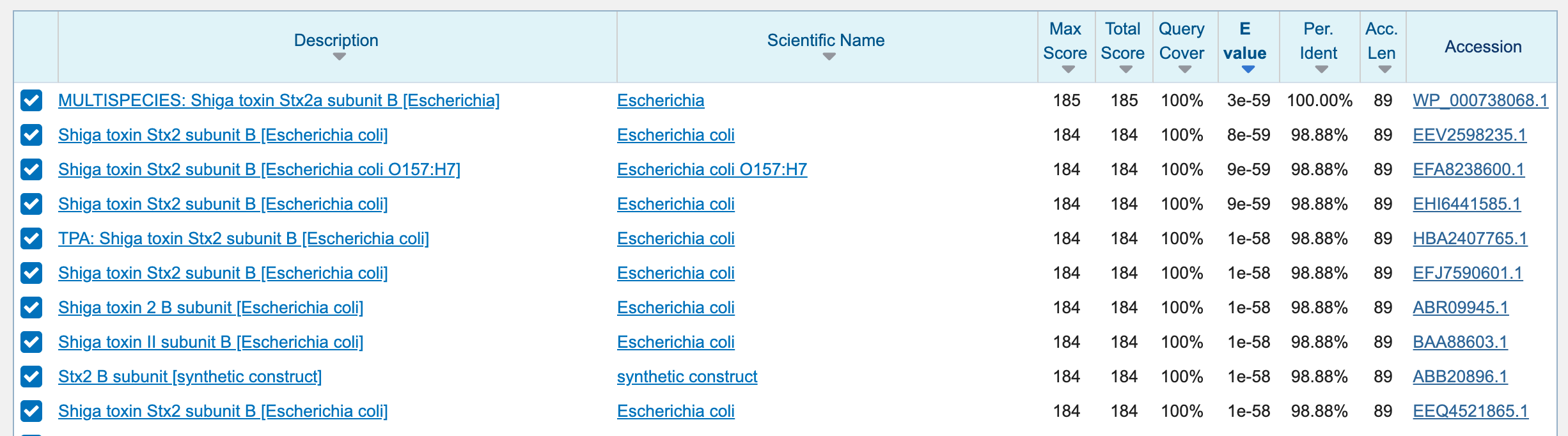
Searching these sequences on the NCBI’s nr databases using BLAST through this website tells us a very sad story:

Real-world examples

Read recruitment forms the backbone of the vast majority of ‘omics investigations and is used from studying subtle responses of organisms in culture to stress to understanding the ecology of environmental microbial populations across the globe. Additional steps in this exercise to demonstrate the recovery of gene-level coverage data are far from hypothetical examples for the sake of discussion, too. For instance, here is a much more realistic example that uses the same exact steps to show the distribution patterns of genes in a single Ruminococcus gnavus genome across human gut metagenomes,

or another one that shows the distribution of genes in two Prochlorococcus marinus genomes across surface ocean metagenomes:

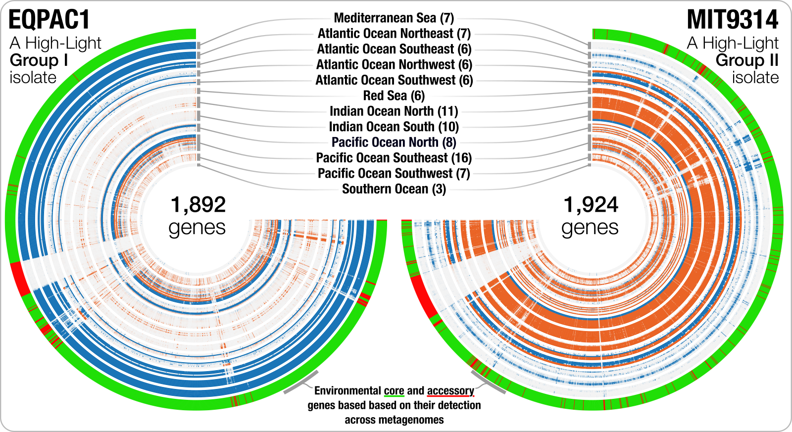
Speaking of real-world examples, if you have millions of genes to profile across hundreds of samples, you probably will not need the visualization of profiles shown in this exercise, but solutions that will report gene coverage statistics directly in flat files. For those applications, you can consider anvi’o programs anvi-profile-blitz or anvi-summarize-blitz.