Vibrio jascida pangenome: a mini workshop

Table of Contents
- Isolate genomes
- Finalizing the list of genomes
- FASTA files to Contigs DBs
- Finalizing the FASTA files
- Generating contigs databases
- Annotating contigs databases
- Taking a quick look at genome stats
- Creating an external genomes file
- Investigating contamination
- Computing the pangenome
- Displaying the pangenome
- Calculating average nucleotide identity between genomes
- Displaying ANI and adjusting it
- Studying the pangenome
The goal of this mini workshop was to compute a Vibrio jascida pangenome using the isolate genomes that were generated during the Microbial Diversity course at the Marine Biological Laboratory in 2018. Essentially, we sat together with the course participants of the Microbial Diversity Course in July 2021 in Woods Hole, and went through the information on this page while discussing what we are seeing and did spontaneous investigations of the pangenome we have computed for Vibrio jascida. We are making this content publicly available in case others wish to play with these data, primarily because why not.
Thanks to the generosity of the Microbial Diversity Course at the MBL, all the novel isolate genomes this mini workshop will be using are now publicly available, and anyone will be able to follow this material on your own anvi’o-installed computers. But if you happen to do something that is much more serious than what is covered here, please consider reaching out to Rachel Whitaker before any publication to discuss the best way forward.
The following material starts with a very brief introduction to the isolates, and work its way through the steps of computing a pangenome using anvi’o. I hope this material will be useful not only to those of you who sat through the workshop at the MBL with me in-person, but also to those of you who run into this material later.
Please feel free to leave a comment at the end of the page or find us on Discord.

This tutorial is tailored for anvi’o v7.1 or later. You can learn the version of your installation by typing anvi-interactive -v. If you have an older version, some things may not work the way they should since we have a few new programs used in this tutorial.
Isolate genomes
Here we will analyze genomes of seven Vibrio jascida populations isolated from various Woods Hole places (including Eel Pond, Marine Resources Center, and the Great Harbor) using complete seawater medium from. This table offers a brief information for each isolate to get back to later:
| Plate Num | Researcher | Source |
|---|---|---|
| 12 | Peggy Lai | Seawater, Great Harbor, Woods Hole |
| 13 | Peggy Lai | Seawater, Great Harbor, Woods Hole |
| 14 | Peggy Lai | Seawater, Great Harbor, Woods Hole |
| 47 | Danielle Campbell | Seawater, Eel Pond, Woods Hole |
| 52 | Brittni Bertolet | ?? |
| 53 | Sarah Schwenck | Coral (from MRC), Woods Hole |
| 55 | Monica E. McCallum | Coral (from MRC), Woods Hole |
Finalizing the list of genomes
Please note that the following few sections will take you through the steps of gathering the FASTA files for genomes we are intersted in and turning them into anvi’o contigs-db files prior to our pangenomic analysis. If you would like to skip these steps completely and start with a collection of contigs-db files directly, please first run either of the following commands depending on which version of anvi’o you’re using.
If you are using anvio-dev, please use this command to download the pre-packaged data:
# download the data pack for v8-dev contigs-db files
curl -L https://cloud.uol.de/public.php/dav/files/XktW549BjTg5ikj \
     -o V_jascida_contigs_dbs.tar.gz
If you are using the stable v8 version of anvi’o, use this command to download the pre-packaged data:
# download the data pack for v8 contigs-db files
curl -L https://cloud.uol.de/public.php/dav/files/7xDdqqXxdtWnpMg \
     -o V_jascida_contigs_dbs.tar.gz
OK. Now you have the pre-packaged data, you can continue with the following commands to unpack the archive:
# unpack it
tar -zxvf V_jascida_contigs_dbs.tar.gz

# go into the new directory
cd V_jascida_contigs_dbs

# take a look at the list of files, you know, as one should always do
ls
Once you are done with them, from here you can jump here to follow the rest of the tutorial.
If you are still here, it means you want to go through each step one by one to go from FASTA files to anvi’o contigs-db files. You are a gem among people.
We will start by downloading the FASTA files for the Vibrio genomes:
# download the pack
curl -L https://cloud.uol.de/public.php/dav/files/LdgMQW6ixzzPKzS \
     -o V_jascida_genomes.tar.gz

# unpack it
tar -zxvf V_jascida_genomes.tar.gz

# go into the new directory
cd V_jascida_genomes

# take a look at what we have in our hands
ls
Please remember these novel genomes are public thanks to the generosity of the Microbial Diversity Course at the MBL and its 2018 participants, Peggy Lai, Danielle Campbell, Brittni Bertolet, Sarah Schwenck, and Monica E. McCallum.
Now we have all the FASTA files for our ‘novel’ Vibrio jascida genomes and in theory we are good to go. But it is always good to try to be a little more inclusive. For instance, to our collection of Vibrio jascida genomes we can include at least one reference genome for this taxon to anchor our pangenome in everyone else’s reality. Indeed, searching on the NCBI for Vibrio jascida does return some complete genomes:
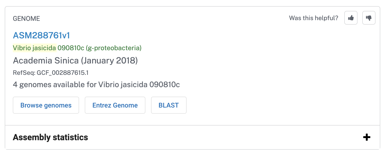
Let’s download the first one:
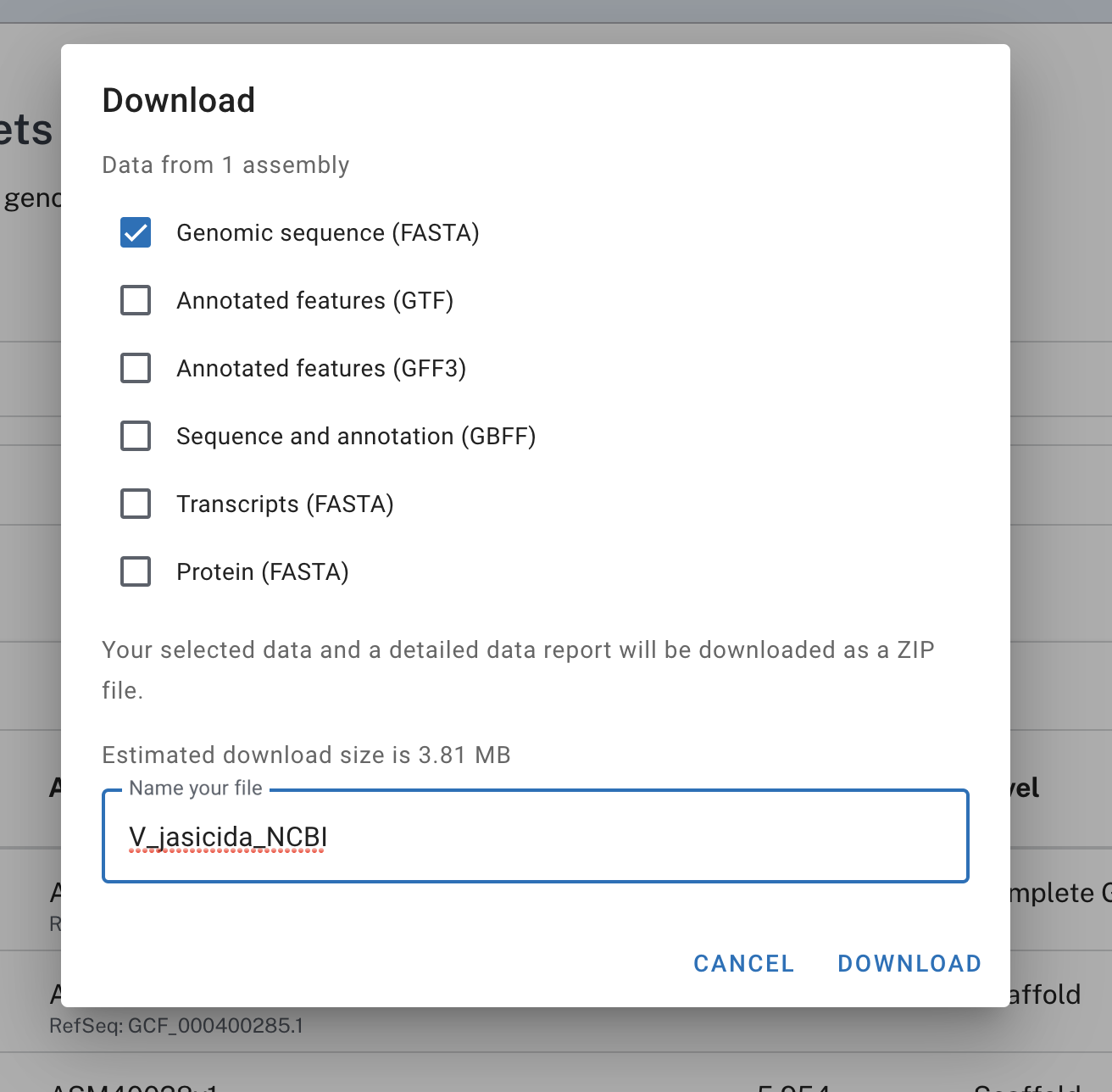
Unzipping the compressed file NCBI sends resulted in a directory with a lot of things in it, but we simply want the FASTA file. This is how I moved that FASTA file of interest into my work directory where all the FASTA files for other Vibrio jascida isolates were living:
mv ~/Downloads/V_jasicida_NCBI/ncbi_dataset/data/GCF_002887615.1/GCF_002887615.1_ASM288761v1_genomic.fna ref_scaffolds.fasta
Please note that the command above may differ for you as a function of a number of things, so please try to figure out where things are if you get an error at this stage. All you want to do is to download a reference genome for our taxon from the NCBI, and move the FASTA file for it into your work directory as ref_scaffolds.fasta.
If you were successful, your work directory should look like this:
ls *fasta

12_scaffolds.fasta
13_scaffolds.fasta
14_scaffolds.fasta
47_scaffolds.fasta
52_scaffolds.fasta
53_scaffolds.fasta
55_scaffolds.fasta
ref_scaffolds.fasta
OK. Now we have all the FASTA files, and we are good to go.
FASTA files to Contigs DBs
For a pangenomic analysis of these genomes we will use anvi’o, an open-source software platform for microbial ‘omics. And anvi’o requires some additional steps for us to be able to work with FASTA files :/
Most analyses in anvi’o start after the conversion of FASTA files into a special anvi’o database called contigs database. So the first order of business is to turn each of these FASTA files into a contigs database.
We can turn a FASTA file into an anvi’o contigs database by running the program anvi-gen-contigs-database. So that is what we need to do that for each one of the FASTA files we have one by one. But a better way to do such repetitive tasks is to put together a for loop using the scripting capabilities of the shell (which we access through our terminal).
To build a for loop, let’s first put our genome names into a text file:
ls *fasta | awk 'BEGIN{FS="_"}{print $1}' > genomes.txt
If you take a look at the contents of this file, you’ll see that it is nothing more than the following:
cat genomes.txt

12
13
14
47
52
53
55
ref
You will see how it will become useful in a second.
Finalizing the FASTA files
Before we go through converting each FASTA file into a contigs database, it is always a great idea to take a look at them to make sure they all make sense. What I mean by looking at them is literally looking at them in a text editor.
For instance, when you do that it becomes immediately clear that the FASTA files assembled from the sequencing of isolates contain many extremely short sequences. Since we are working with cultured organisms and expect high-quality assemblies, it is a good idea is to start by removing sequences that are too short since they may be coming from low-abundance contaminants that didn’t assemble well and/or influence how gene clusters are formed.
There are multiple ways to remove short sequences. But here we will go through each entry in our genomes.txt file, and use the program anvi-script-reformat-fasta create copies of each FASTA file without the sequences that are less than 2,500 nucleotides:
for g in `cat genomes.txt`
do
    echo
    echo "Working on $g ..."
    echo
    anvi-script-reformat-fasta ${g}_scaffolds.fasta \
                               --min-len 2500 \
                               --simplify-names \
                               -o ${g}_scaffolds_2.5K.fasta
done
Generating contigs databases
Now we have our final, anvi’o-compatible FASTA files, it is time to generate anvi’o contigs databases using the program anvi-gen-contigs-database:
for g in `cat genomes.txt`
do
    echo
    echo "Working on $g ..."
    echo
    anvi-gen-contigs-database -f ${g}_scaffolds_2.5K.fasta \
                              -o V_jascida_${g}.db \
                              --num-threads 4 \
                              -n V_jascida_${g}
done
Annotating contigs databases
An anvi’o contigs-db is a talented form of a FASTA file, and in addition to our genome sequences, it can hold a lot of additional information per genome. Such as gene calls, sequence k-mer frequencies, gene functions, and so on. Here we can use some relevant anvi’o programs, such as anvi-run-hmms, anvi-run-ncbi-cogs, anvi-scan-trnas, anvi-run-scg-taxonomy, to identify bacterial single-copy core genes, ribosomal RNAs, transfer RNAs among our contigs, and annotate our genes with functions (note that we are now going through each file that ends with ‘.db’, rather than entries in the genomes.txt):
for g in *.db
do
    anvi-run-hmms -c $g --num-threads 4
    anvi-run-ncbi-cogs -c $g --num-threads 4
    anvi-scan-trnas -c $g --num-threads 4
    anvi-run-scg-taxonomy -c $g --num-threads 4
done
Taking a quick look at genome stats
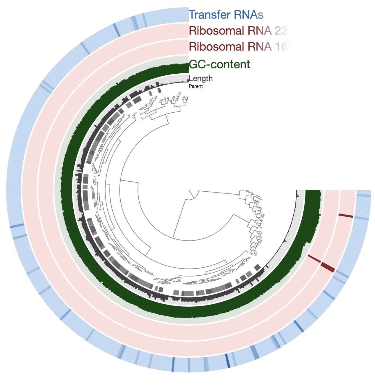
If you are here, it means you have your contigs-db files ready and you are ready to jump into the pangenomics. But first, let’s take a look at the simple features of these genomes we have using the program anvi-display-contigs-stats:
anvi-display-contigs-stats *db
Running this pulls this display up on my browser:

There is a lot to discuss here, so let’s take a moment and try to make sense of this information here.
Creating an external genomes file
This is not necessarily a standard step of turning FASTA files to contigs databases, but when we need to work with a bunch of contigs databases in anvi’o, we use a special file called external-genomes to describe them all together in one place as a logically relevant group of contigs databases (in case you are curious, yes there also is an internal-genomes file format). So let’s create one here so we can use it for our downstream analyses.
The structure of the external-genomes file is simple: it is a two-column TAB-delimited file. One can easily create it using EXCEL or any kind of text editor. But anvi’o comes with a script, anvi-script-gen-genomes-file to create one from all the contigs databases found in a directory. So let’s use that to generate an external genomes file:
anvi-script-gen-genomes-file --input-dir . \
                             -o external-genomes.txt
You can take a look at the resulting file to see how simple it is.
Investigating contamination
In theory, everything is ready at this point for us to compute a pangenome. But when one is dealing with sequence data, nothing can ever be truly ready for anything in practice. I learned over the years that every time I look at things more carefully I find more things to improve. There is no end to it and we often have to call it a day and move on. But this is the last checkpoint before we turn our genomes into a pangenome, so it is a good idea to invest a little more time to see if there is something that would REALLY upset us later.
We can start by taking a quick look at the level of completion of our genomes using the program anvi-estimate-genome-completeness, which, like many anvi’o programs, accepts external-genomes as an input:
anvi-estimate-genome-completeness -e external-genomes.txt
And voila:
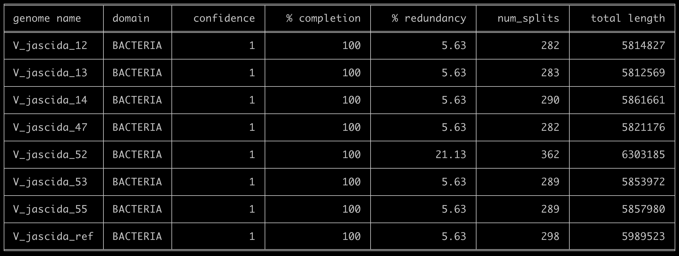
This output clearly shows that there is something fishy going on with V_jascida_52. It has more redundancy than others, it is larger in size than others, etc. This can be due to some sort of contamination, but how can we be sure? One way to do it is to take a more careful look at this genome by visualizing it through anvi-interactive, and perhaps remove some contigs from it if necessary.
Visualizing contigs for refinement
If you were to look at the help menu of anvi-interactive you would realize that this program requires an anvi’o profile database. Which we do not have, since we did not profile anything.
Profiling in anvi’o typically makes sense of read recruitment results, and we have not conducted any read recruitment here since we did not have access to the raw sequencing data of these isolates.
But while the program anvi-refine requires a BAM file as an input, we still can generate a blank profile without any mapping results using the flag --blank:
anvi-profile -c V_jascida_52.db \
             --sample-name V_jascida_52 \
             --output-dir V_jascida_52 \
             --blank
OK. Now we are ready to use anvi-interactive:
anvi-interactive -c V_jascida_52.db \
                 -p V_jascida_52/PROFILE.db
Which shows us this display:
The organization of contigs based on tetranucleotide frequency shows clear signs of contamination, but we are able to identify a set of contigs that we are relatively more confident to represent the true V. jascida genome we are interested in. In my opinion this is how it looks like:
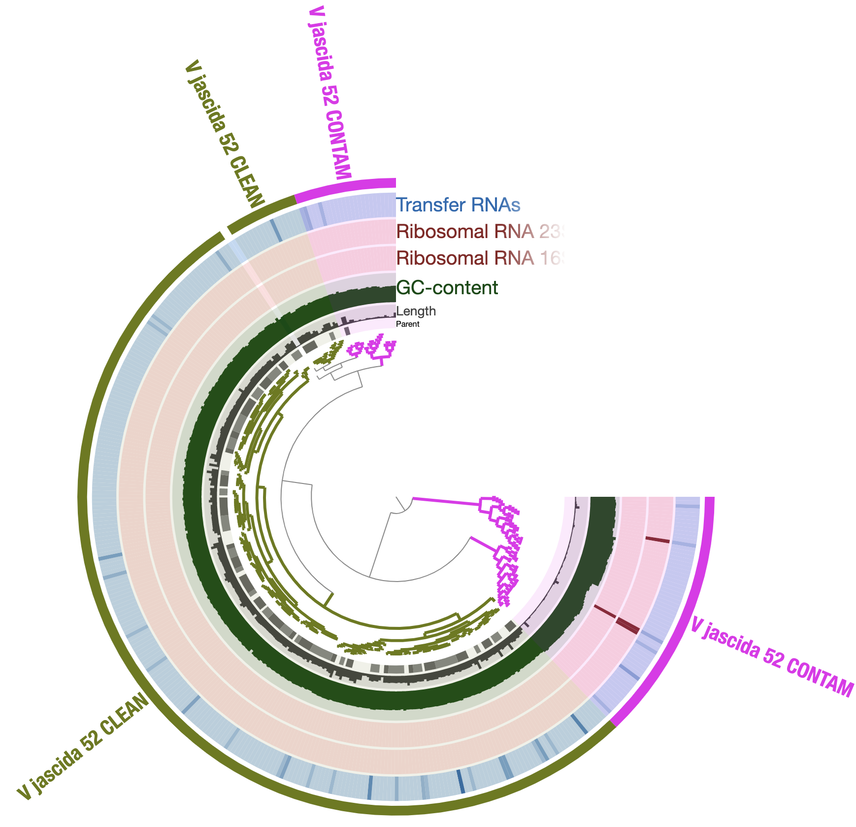
We can even talk about what is contaminating:
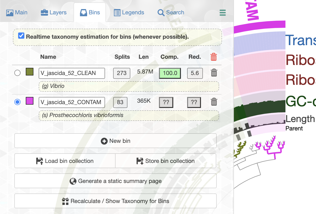
So it is clear that we don’t want to include those contaminating genes in our analysis and we should only work the But how to get those sequences we marked as V_jascida_52_CLEAN. But how do we get those sequences?
Splitting a genome
Getting out the clean sequences from this will be much easier than you probably think, but it requires some introduction to some of the anvi’o lingo for which we don’t have time or space. That said, here is a very brief blurb: we have stored our bins into a collection called default using the store bin collection button in the previous screenshot (the collection name doesn’t really matter, we could call it anything). Having a collection in an anvi’o profile database (which is stored in our blank profile database in this case), enables us to access sequences in those bins in different ways. If you would like to have an idea, you can take a look at all the anvi’o programs that can work with a collection artifact.
One of those programs that can use a collection is the program anvi-split, which does something we really need: splits a contigs database into smaller ones each of which individually represent a single bin in a collection. So we can run it on our poor Vibrio jascida #52:
anvi-split -p V_jascida_52/PROFILE.db \
           -c V_jascida_52.db \
           -C default \
           -o V_jascida_52_SPLIT
The contigs-db for the ‘cleaned up’ V. jascida #52 is now here in my work directory:
V_jascida_52_SPLIT/V_jascida_52_CLEAN/CONTIGS.db
Updating the external genomes file
Now we have a better contigs database for V. jascida #52, we want to have a new external-genomes file where the old V. jascida #52 is replaced with the cleaner one. One quick way to do that is the following:
sed 's/V_jascida_52.db/V_jascida_52_SPLIT\/V_jascida_52_CLEAN\/CONTIGS.db/g' external-genomes.txt > external-genomes-final.txt
Which creates a new file called external-genomes-final.txt that we can use for downstream analyses. Before we move on, let’s take a look at the difference between the two sets of contigs databases using anvi-estimate-genome-completeness just to be sure:
anvi-estimate-genome-completeness -e external-genomes.txt
anvi-estimate-genome-completeness -e external-genomes-final.txt
Computing the pangenome
The first step of computing a pangenome is to generate a yet-another anvi’o artifact: genomes storage, which essentially merges all the contigs databases into a single, leaner file, so pangenomes can be made publicly available. The program anvi-gen-genomes-storage does that for us by taking in an external-genomes file:
anvi-gen-genomes-storage -e external-genomes-final.txt \
                         -o V_jascida-GENOMES.db
This step took 6 seconds on my laptop.
Then, we can use the program anvi-pan-genome to compute the pangenome:
anvi-pan-genome -g V_jascida-GENOMES.db \
                --project-name V_jascida \
                --num-threads 4
This step took 4 minutes on my laptop.
Displaying the pangenome
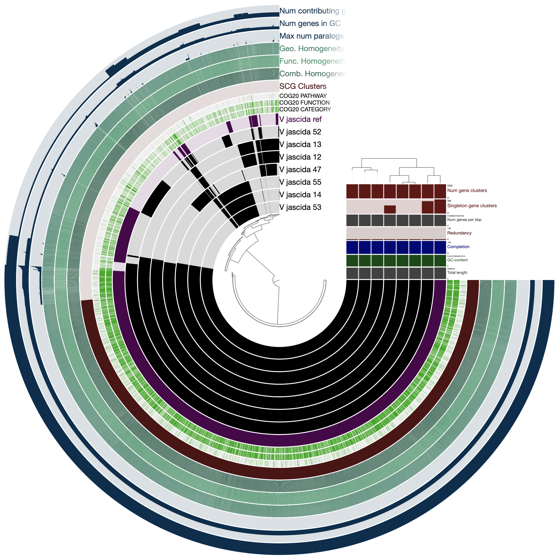
We can now visualize this pangenome the program anvi-display-genome and start discussing what we see.
anvi-display-pan -p V_jascida/V_jascida-PAN.db \
                 -g V_jascida-GENOMES.db
The command above gives us this ugly (yet interactive) display:

There are many things that can be done here, and covering all the features of the interface would be almost impossoble. But let’s do a few things to improve our understanding of the members of this pangenome. First, let’s change the background color of the reference genome so we see it clearly.
For that we first mark it in the ‘main panel’ so it is easy to see which genome it is:

And then change the background color before re-drawing it:

When we redraw, this is what we see:
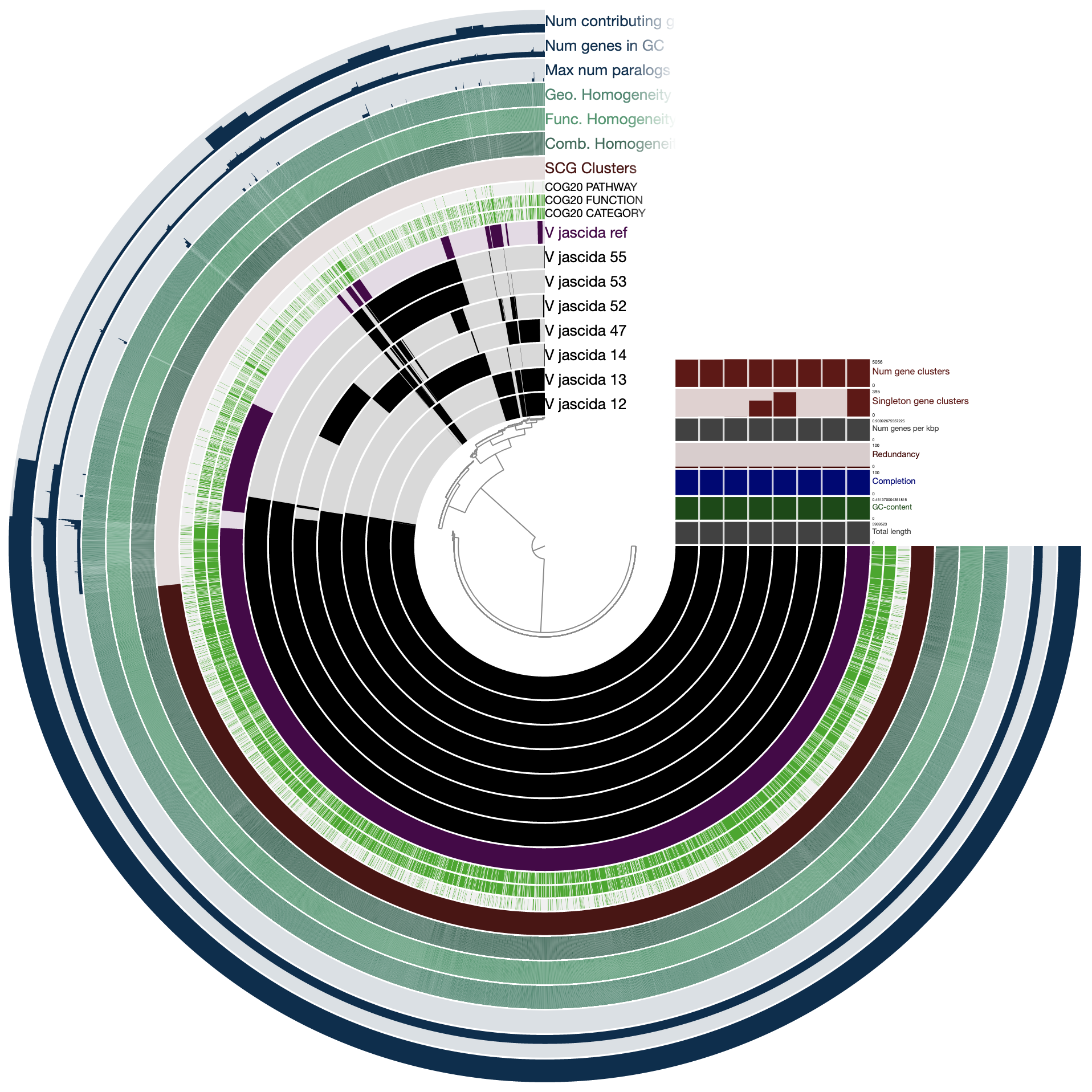
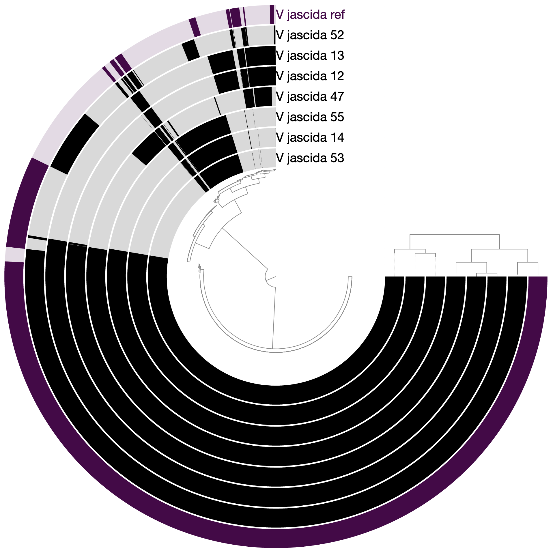
As you can see the way genomes are ordered in this display follows the alphabetical order. Gene clusters, however, don’t seem to care much about the way we named the genomes. The next thing we can do is to switch to a more meaningful order using the Layers panel:
Drawing again, gives us this:
Things are slowly coming together, but the display is just way too busy. We can remove all those additional layers for now and then turn them on for our discussions. First the additional data layers for items:
Then the additional data for layers:
OK. Looks much better.
Calculating average nucleotide identity between genomes
One question that display can not answer to what extent the associations between genomes are predicted by the average nucleotide identity between each genome. But we can easily recover that by using the program anvi-compute-genome-similarity to calculate ANI between genomes, and also add that information to the pangenome:
Before killing your server to run this command, you may want to store your state :)
anvi-compute-genome-similarity --external-genomes external-genomes-final.txt \
                               --program pyANI \
                               --output-dir ANI \
                               --num-threads 6 \
                               --pan-db V_jascida/V_jascida-PAN.db
The successful completion of this will update our pangenome.
Displaying ANI and adjusting it
We can re-display the same pangenome, now with ANI values in it, using anvi-display-genome:
anvi-display-pan -p V_jascida/V_jascida-PAN.db \
                 -g V_jascida-GENOMES.db
But to actually display ANI values, we need to turn on what we wish to display from the Layers tab:
Although clicking redraw may yield a rather disappointing discovery o_O
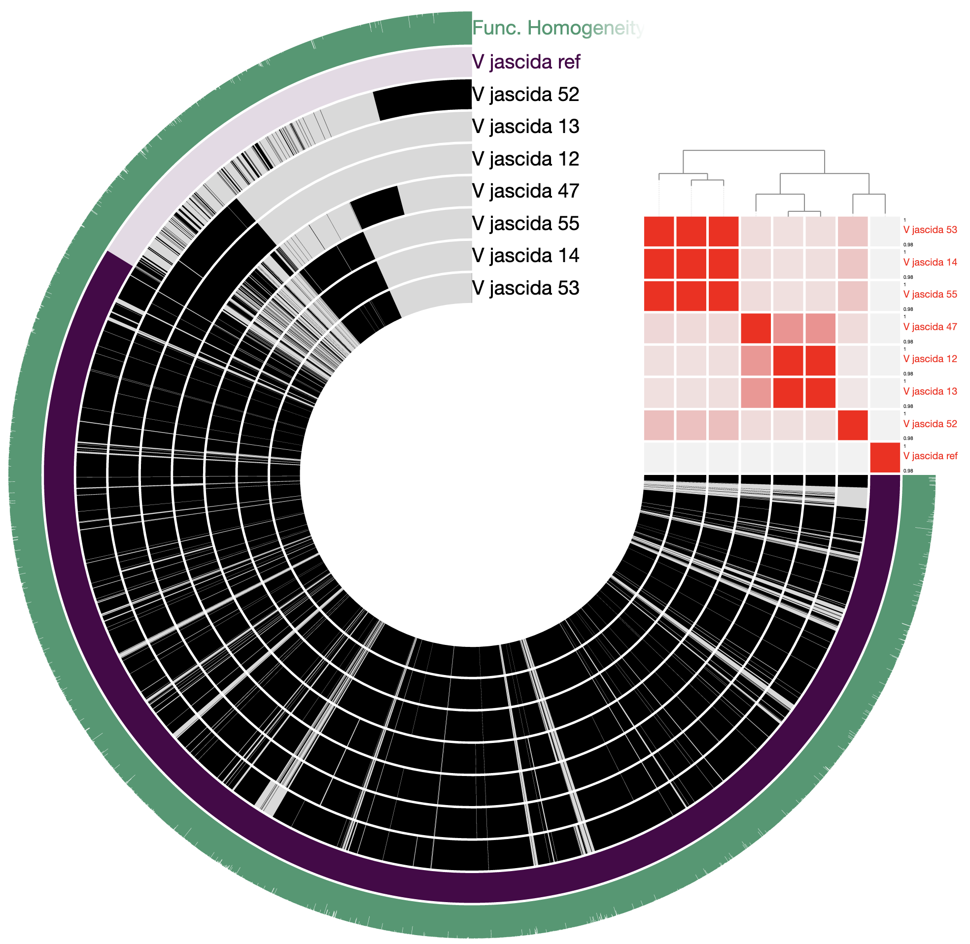
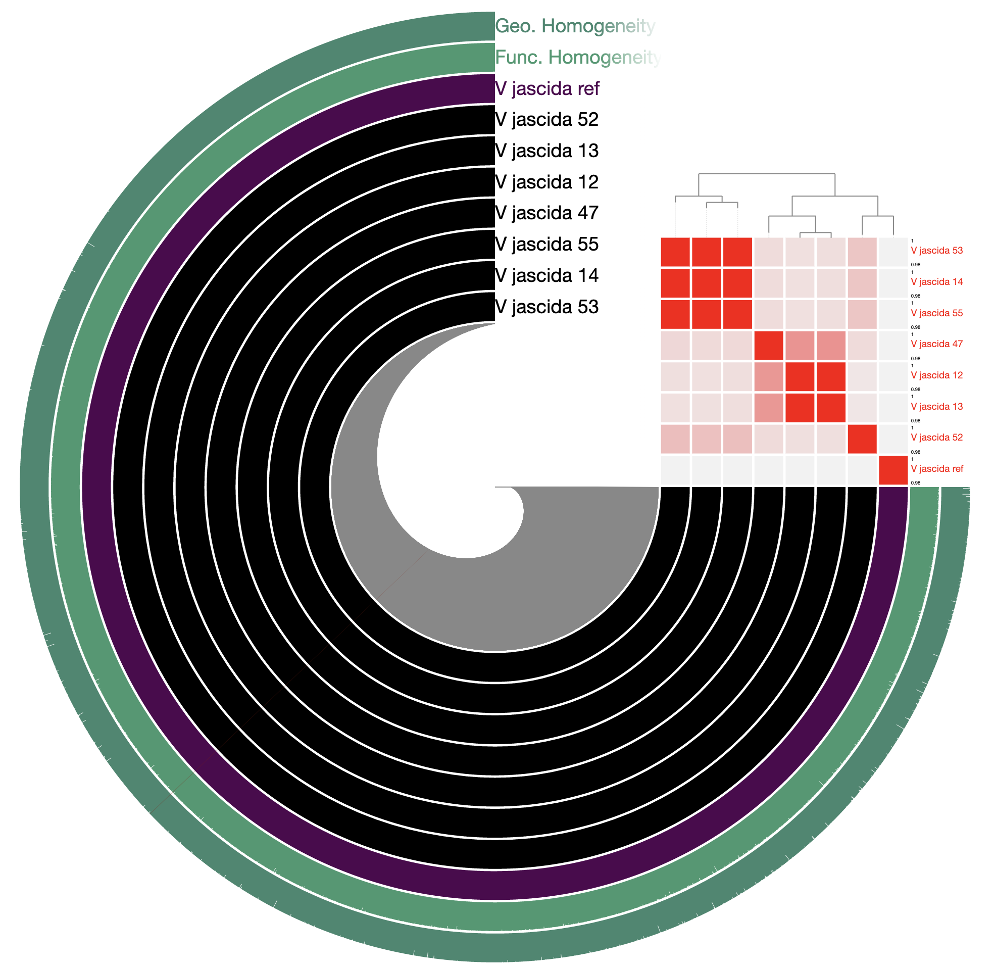
But do not despair. This is due to the fact that the default min-max values of ANI values are set to 70% to 100%, and our genomes way too closely related for those numbers to make sense. Since they resolve to the same ‘species’, 95% ANI is a much better cutoff than 70% to start with.
One can in fact quickly adjust these values:
98% it is. With that, things make a little more sense:
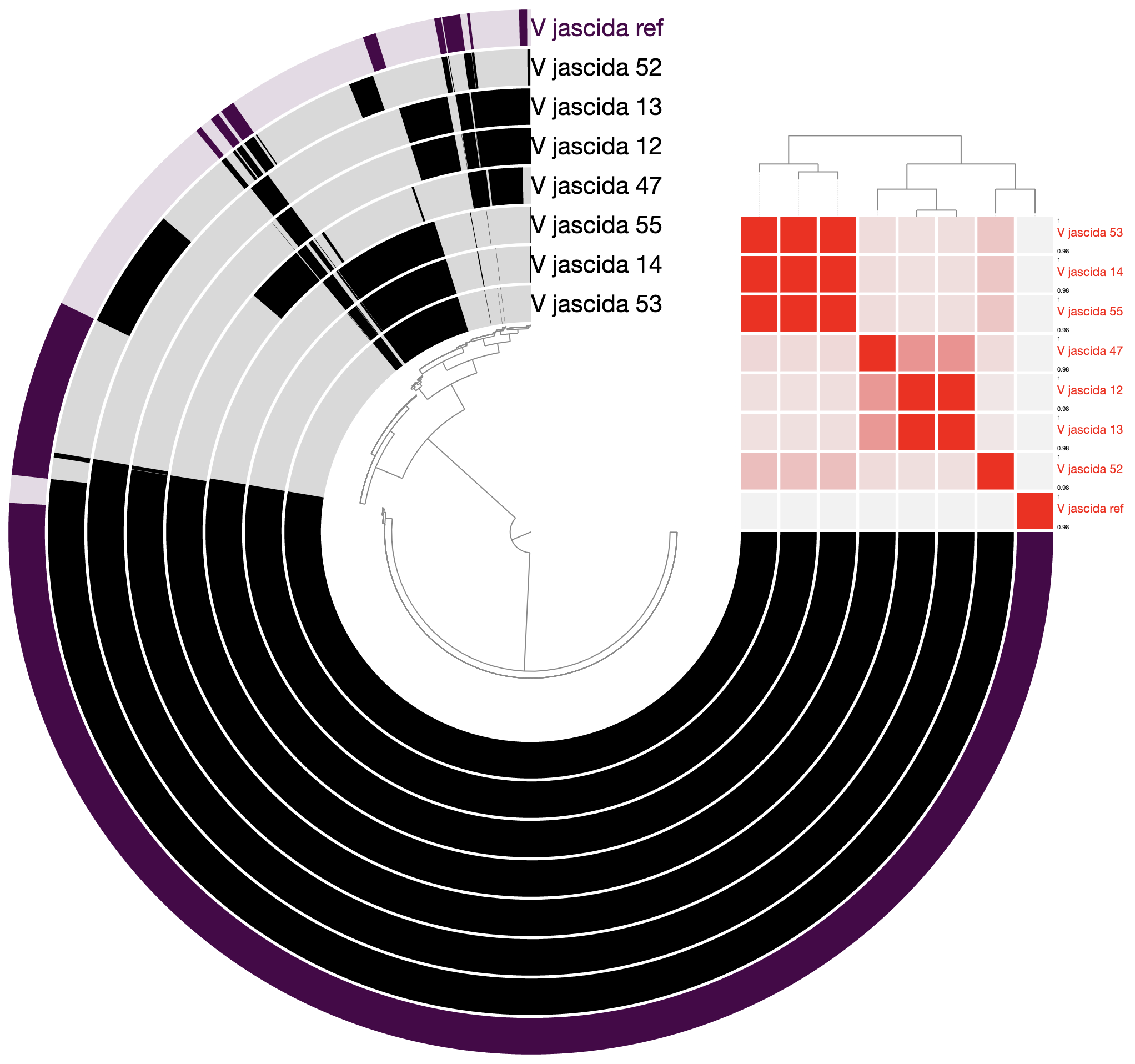
Studying the pangenome
Perhaps this is a good moment to stop and discuss what we are seeing in the light of how these isolates relate to one another:
| Plate Num | Researcher | Source |
|---|---|---|
| 12 | Peggy Lai | Seawater, Great Harbor, Woods Hole |
| 13 | Peggy Lai | Seawater, Great Harbor, Woods Hole |
| 14 | Peggy Lai | Seawater, Great Harbor, Woods Hole |
| 47 | Danielle Campbell | Seawater, Eel Pond, Woods Hole |
| 52 | Brittni Bertolet | ?? |
| 53 | Sarah Schwenck | Coral (from MRC), Woods Hole |
| 55 | Monica E. McCallum | Coral (from MRC), Woods Hole |
There are MANY ways to perform exploratory analyses or test hypotheses once one reaches to this stage. I would like everyone to take 30 minutes with the pangenome to find their own stories in it. But here are some quick tips that you may find beneficial.
Inspecting amino acid sequence alignments

Binning gene clusters
Changing how gene clusters are ordered
For instance, an ‘enforced synteny’ using the reference genome will change your display, where gene clusters will be ordered to respect the synteny of the genes they contain in the reference genome:
Selecting a range of gene clusters

Searching for functions

Searching using gene cluster filters
Storing a collection
Storing a collection is an important step since the concept of collection is important for anvi’o.
Splitting a pangenome
Do you remember the program anvi-split that we used to split a genome into pieces? Well, the same program can split a pangenome, too, because that’s how anvi’o rolls. If you were to be interested in focusing ONLY on the single-copy core gene clusters we stored as a collection in the previous gif, you could split it from the pan database into its standalone project.
If you don’t remember collections stored in your pangenome, you can always use the program anvi-show-collections-and-bins:
anvi-show-collections-and-bins -p V_jascida/V_jascida-PAN.db

Collection: "my_collection"
===============================================
Collection ID ................................: my_collection
Number of bins ...............................: 2
Number of splits described ...................: 5,131
Bin names ....................................: SCGs, Singletons
OK, so we want the SCGs bin from the collection my_collection. Here comes the anvi-split:
anvi-split -p V_jascida/V_jascida-PAN.db \
           -g V_jascida-GENOMES.db \
           --collection-name my_collection \
           --bin-id SCGs \
           --output-dir SPLIT
And here we go:
anvi-display-pan -p SPLIT/SCGs/PAN.db \
                 -g V_jascida-GENOMES.db
It is boring because everything is a single-copy core here. But there are indeed very interesting things to do. If we have time here during the workshop, Meren will show an extremely high-resolution phylogenomics analysis using subtly varying single-copy core genes.
Summarizing the pangenome
This effectively gives you a huge TAB-delimited file that describes everything you see on your pangenome. It is quite a critical output.
While I would strongly recommend you to use the anvi’o command line program anvi-summarize to generate a static output file for your pangenome, you can also do it through the interface:
Perhaps this is a good moment to take a look at the summary output, and open the summary of gene clusters in EXCEL or R.
Sharing the pangenome with others
The anvi-summarize step essentially generates an output directory with an index.html file that can be opened on any browser, and enables you to share your pangenome as a supplementary data item in any publication.
Another option, especially if you would like to feel like the year 2021 has finally arrived, you can shre your pangenome in a fully reproducible and interactive way. For that (1) create a new directory, (2) copy into this directory the two essential files, V_jascida/V_jascida-PAN.db and V_jascida-GENOMES.db, (3) compress the directory (i.e., tar/gz it), (4) upload it to Zenodo or FigShare, and (5) include the DOI for this item in your data availability section of your publication.
Thank you for your time! Please let me or others know if you have any suggestions!