


Table of Contents
- Prepare your Mac
- Introduction to microbial ecology
- Crassphage
- Short introduction to metagenomic sequencing
- Using a mapping approach to assess the occurence of crassphage in metagenomes
- Working on the University of Chicago’s midway computer cluster
- Using snakemake to run the analysis steps
- Predicting a host for crassphage
- Loading the data
- Pre-processing the data
- A clustering approach to identifying a host
- Training a random forest regression model
- Model Results
- Exploring the mapping results with “gene mode”
- The global distribution of phicrass001

This workshop was developed as part of the BRI class for the University of Chicago Biophysical Sciences Graduate Program first year students in the fall quarter of 2018. The workshop was planned for 20 hours in-class, and the students were expected to do additional work on assignment outside of class hours.
The general goals of this workshop are:
- Introduce the students to some of the microbial ecology and microbial omics type of work that is being done in the Meren Lab.
- Learn a new practical tool (snakemake) through some hands-on experience.
The specific goals of this workshop are:
- Get familiar with some basic questions of microbial ecology.
- Learn how questions of microbial ecology are addressed using ‘omics approahces through the example of crassphage.
- Learn, through the example of snakemake, how workflow managment tools help us streamline the analysis of large collection of genomic samples.
- Learn how large datasets could serve as an input to machine learning algorithms, and help us address questions of microbial ecology.
Prepare your Mac
For this workshop you are required to install the following things:
brew
I recommend installing homebrew. There are many ways to install anvi’o, but using the brew command is the easiest.
python
Your Mac already came with python, but I would recommend isntalling a different python with brew (specifically, you would need python3).
I also recommend installing the jupyter notebook. You can refer to the jupyter installation instructions page.
anvi’o (and some dependencies)
Before we install anvi’o, we need to install the following third party software: samtools, prodigal, HMMER, GSL, Numpy, and Cython.
After we have all of the dependencies, we can install anvi’o
Introduction to microbial ecology
The introduction will include a lecture by Dr. Eren. Slides will be available here as soon as possible.
Crassphage
Slides for the introduction to crassphage and the workshop plan could be downloaded here.
The background includes review of these crassphage related papers:
Short introduction to metagenomic sequencing
In this workshop we will be working with pair-end short reads that were produced by an Illumina sequencer. If you are not familiar with it, I recommend reffering to this 5 minutues video by Illumina that explains the sequencing process. In class, we will also go over this short presentation.
Using a mapping approach to assess the occurence of crassphage in metagenomes
Following a similar approach to the one in Dutilh et al., we will use read recruitment to quantify the occurence of crassphage in gut metagenomes.
We will use metagenomes from the following studies: The Human Microbiome Project Consortium 2012 (USA), Rampelli et al. 2015 (Tanzania), Qin et al. 2012 (China), and Brito et al. 2016 (Fiji). This will allow us to get some minimal understanding of the global distribution of crassphge.
In this workshop we will use a total of 434 metagenomes, in this section of the workshop we will only analyze a small portion of these metagenomes. The purpose is to understand what are the steps that are required for this analysis, and to understand that to do each step manually is not a good idea. Hence, later, we will use a snakefile to analyze the rest of the samples. Notice that I directly shared files with the students, so if you are not a student of the workshop, but interested in getting these files, please contact me. In addition, in this workshop we also use the sequence of phicrass001, which I obtained directly from Andrey Shkoporov, and hence I will not make it available here.
Assignment - check for crassphage in samples
I provided you with 12 bam files (3 from each country). Each student will pick three samples, and go through the following steps in order to view these bam files with anvio. To keep things simple, I provide you with bam files, and hence, you are spared from taking many of the analysis steps (e.g. quality filtering of the metagenomes, mapping of short reads to the reference genome, formatting of mapping results, etc.)
generate a contigs database
This step proccesses the reference fasta file that we are using. In this case, it is the genome of crassphage (which could be downloaded here). You can learn more by reffering to the help menu or to this section of the anvio metagenomics tutorial. To generate the database run:
anvi-gen-contigs-database -f crassphage.fasta -o crassphage-contigs.db -n crassphage
profile the bam file
The bam file contains the alignment information for the short reads against the reference genome. anvi-profile computes variouos stats from the alignment, and paves the way to the visualization of this information. This step is performed for each sample separately. For more information refer to the help menu and to this section of the anvio metagenomics tutorial.
To run anvi-profile for a bam file:
anvi-profile -i PATH/TO/BAM_FILE.bam -c crassphage-contigs.db
merge the bam files
After all the individual profiling steps are done, we merge these profiles together so that we can visualize them. For more information refer to the help menu, or to this section of the anvio metagenomics tutorial.
anvi-merge */PROFILE.db -o SAMPLES-MERGED -c crassphage-contigs.db --skip-concoct-binning
Notice that I added the flag --skip-concoct-binning, since we are not interested in binning in this case. If you don’t know what binning is, that’s ok, it’s not important for this workshop.
After these steps are done. use anvi-interactive to view the results. Do you see any trend in the global distribution of crassphage?
In class, we will also use the --gene-mode of anvi-interactive to look at the occurence of the crassphage genes.
We will also use the inspect option of the interface to look at SNVs.
Working on the University of Chicago’s midway computer cluster
Bioinformatic analysis often are done on a cluster of computers (aka supercomputer) in order to allow for a faster computation, and since you don’t usually want to leave something running on your computer for days. In order to perform our analysis we will get familiar with the following things:
- Connecting to a remote host using
sshand transfering files usingscp. - Understand the concept of queue managing software, and learn to use slurm (the queue managing software used on midway).
- In a later section we will also learn things related to running snakemake on a cluster:
- work with
screen. - learn how to configure snakemake to submit jobs to the queue.
- work with
Working with a remote host
Typically, a cluster computer is configure so that it is accessed through a head node. The headnode is just a normal computer, and it is only used for accessing purposose, so we connect to it using ssh, and we submit our jobs to queue. In other words, we don’t want to actually run anything on it.
In order to connect midway, you can read the details on the RCC website, but basically you run (we will use midway2):
ssh YOUR_CNET_ID@midway2.rcc.uchicago.edu
And then you enter your password.
Making your life a little easier when working with a remote host
There are a few things we can do to make our life easier when working on a remote host.
The first thing is use an RSA key to avoid having to insert our password every time we connect. Simply follow the instructions here:
Using snakemake to run the analysis steps
Since bioinformatics tends to include many steps of analysis, it is becoming more and more popular to use workflow management tools to perform analysis. Two popular tools are nextflow and snakemake. Here we will get familiar with snakemake and write a simple workflow to run the steps from above.
We will go through this introduction to snakemake from Johannes Koester (the developer of snakemake). But the best way to become familiar with snakemake is to refer to the online docummentation.
Assignment - write a snakefile to excecute the same steps from earlier
We will write a snakefile that accepts a list of bam-files with the path to each bam file, and a name for each sample. We will then use this snakefile to run these steps for all the 434 samples from the global studies.
Feel free to go about this in any way you want. I recommend using pandas to read a tab-delimited file with a name for each sample, and the path to the bam file.
In addition, in this section of the workshop, we will learn to work with a computer cluster. We will use Midway.
Using “screen” to run stuff
We always start our work by initiating a screen session. If you are not familiar with what this is, basically, we use it here because we are running something that requires no user interaction for a long time on a remote machine (e.g. a cluster head node).
screen -S mysnakemakeworkflow
After the workflow is running you simply click ctrl-A followd by D to detach from the screen. If you want to check the status of your workflow, then to reconnect to your screen use:
screen -r mysnakemakeworkflow
And when you want to kill it use ctrl-D (while connected to the screen).
At any given time you can see a list of all your screens this way:
screen -ls
Simple, but extremely efficient.
Predicting a host for crassphage
Similar to the approach in Dutilh et al., we will use the abundance of crassphage in metagenomes along with the abundance of various taxons, to try to predict a host for crassphage. In order to asses the occurence of various bacteria in our collection of metagenomes, I ran krakenHLL. And the results for the species and genus levels are provided in samples-species-taxonomy.txt, and samples-genus-taxonomy.txt, respectively. We will now examine two alternative approaches to predicting a host for crassphage. Both of these approaches rely on the idea that the host of crassphage should have a positively correlating occurence with crassphage. A jupyter notebook with all the steps for this part of the workshop is available here.
Loading the data
import pandas as pd

tax_level = 'species'
data_file = 'samples-'+ tax_level + '-taxonomy.txt'
target_file = 'crassphage-samples-information.txt'

raw_data = pd.read_csv(data_file, sep='\t', index_col=0)
raw_target = pd.read_csv(target_file, sep='\t', index_col=0)
But before we try to predict anything from the data, we will pre-process the data.
Pre-processing the data
First we remove all the samples that don’t have crassphage (crassphage negative samples).
all_samples = raw_data.index
crassphage_positive_samples = raw_target.index[raw_target['presence']==True]
print('The number of samples in which crassphage was detected: %s' % len(crassphage_positive_samples))
crassphage_negative_samples = raw_target.index[raw_target['presence']==False]
print("The number of samples in which crassphage wasn't detected: %s" % len(crassphage_negative_samples))
# Keep only positive samples
samples = crassphage_positive_samples
The number of samples in which crassphage was detected: 80
The number of samples in which crassphage wasn't detected: 240
Ok, so there are a lot more negative samples than positive samples.
Let’s look at where are the positive samples coming from.
for o in ['USA', 'CHI', 'FIJ', 'TAN']:
    a = len([s for s in crassphage_positive_samples if s.startswith(o)])
    b = len([s for s in all_samples if s.startswith(o)])
    c = a/b * 100
    print('The number of crassphage positive samples from %s is %s out of total %s (%0.f%%)' % (o, a, b, c))
The number of crassphage positive samples from USA is 53 out of total 103 (51%)
The number of crassphage positive samples from CHI is 16 out of total 46 (35%)
The number of crassphage positive samples from FIJ is 11 out of total 167 (7%)
The number of crassphage positive samples from TAN is 0 out of total 8 (0%)
We can see that crassphage is most prevalent in the US cohort, but also quite common in the Chinese cohort. Whereas it is nearly absent from the Fiji cohort, and completely absent from the eight hunter gatherers from Tanzania.
Normalizing the data
The krakenhll output is in counts, so we will normalize this output to portion values, so that the sum of all taxons in a sample will be 1. We will also normalize the crassphage values, but since we don’t have the needed information to translate these values to portion of the microbial community, we will just make sure that the values are between zero and one, by deviding by the largest values.
normalized_data = raw_data.div(raw_data.sum(axis=1), axis=0)
normalized_target = raw_target['non_outlier_mean_coverage']/raw_target['non_outlier_mean_coverage'].max()
Removing rare taxons
We will remove the taxons that don’t occur in at least 3 of the crassphage positive samples. The reasoning here is that a taxon that occurs so uncommonly is more likely to be an outcome of spuriuous misclassification, and would anyway contribute very little to a successful classifier.
occurence_in_positive_samples = normalized_data.loc[crassphage_positive_samples,]
qualifying_taxons = normalized_data.columns[(occurence_in_positive_samples>0).sum()>3]
portion = len(qualifying_taxons)/len(normalized_data.columns) * 100
print('The number of qualifying taxons is %s out of total %s (%0.f%%)' % (len(qualifying_taxons), \
                                                                         len(normalized_data.columns), \
                                                                         portion))

data = normalized_data.loc[samples, qualifying_taxons]
target = normalized_target[samples]
The number of qualifying taxons is 69 out of total 273 (25%)
A clustering approach to identifying a host
We will try a hierarchical clustering approach similar to what was done in the crassphage paper.
First we will merge the data together (i.e. add the crassphage coverage as a column to the kraken table):
# add the crassphage column
merged_df = pd.concat([data, target], axis=1)
# Changing the name of the crassphage column
merged_df.columns = list(merged_df.columns[:-1]) + ['crassphage']
# Write as TAB-delimited

# anvi'o doesn't like charachters that are not alphanumeric or '_'
# so we will fix index and column labels
import re
f = lambda x: x if x.isalnum() else '_'
merged_df.columns = [re.sub('\_+', '_', ''.join([f(ch) for ch in s])) for s in list(merged_df.columns)]
merged_df.index = [re.sub('\_+', '_', ''.join([f(ch) for ch in s])) for s in list(merged_df.index)]

# Save data to a TAB-delimited file
merged_df.to_csv(tax_level + '-matrix.txt', sep='\t', index_label = 'sample')
Now we leave the python notebook and go back to the command line.
There are a few steps needed to be done in order to visualize this data with anvio (described here), but we will use a snakefile I wrote to streamline thie process. This snakefile requires a config file, which is available here.
If you try to use this snakefile on your own data, beware that this snakefile is not highly robust, and might not work for your case of interest.
snakemake -s snakemake_to_generate_manual_interactive_interface_for_tabular_data.snake --configfile config.json
I also created a slightly nicer view of the data which we could import to the manual profile database (the state file is available here):
anvi-import-state -p 00_ANVIO_FIGURE/PROFILE.db \
                  -s crassphage-host-predict-default-state.json \
                  -n default
Lastly, I made some selections in the interface to highlight the potential hosts. Let’s load the collection I created (available here: collection file, and collection info file)
anvi-import-collection -p 00_ANVIO_FIGURE/PROFILE.db \
                       -C default \
                       --bins-info crassphage-host-predict-default-collection-info.txt \
                       crassphage-host-predict-default-collection.txt
Now we can view the results:
anvi-interactive --manual \
                 -d species-matrix.txt-transposed-item-names-fixed \
                 -p 00_ANVIO_FIGURE/PROFILE.db \
                 -t 00_ANVIO_FIGURE/crassphage_species.newick \
                 --title crassphage_species
This is it what it looks like:
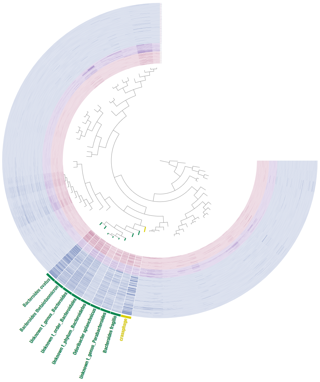
We can see that this includes members and close relatives of the Bacteroides genus, hence we get a similar result to Dutilh et al.
Training a random forest regression model
Similar to the clustering approach, we will use each one of the taxonomy tables to train a Random Forrest regression model, and see if we can predict possible hosts for crassphage. In preparing this part of the tutorial, I advised this blog post by Fergus Boyles.
The input data for the model are the normalized abundances from KrakenHLL, and the target data for prediction is the normalized non-outlier mean coverage of crassphage.
from sklearn import ensemble
n_trees = 64
RF = ensemble.RandomForestRegressor(n_trees, \
                                    oob_score=True, \
                                    random_state=1)

RF.fit(data,target)
RandomForestRegressor(bootstrap=True, criterion='mse', max_depth=None,
           max_features='auto', max_leaf_nodes=None,
           min_impurity_decrease=0.0, min_impurity_split=None,
           min_samples_leaf=1, min_samples_split=2,
           min_weight_fraction_leaf=0.0, n_estimators=64, n_jobs=1,
           oob_score=True, random_state=1, verbose=0, warm_start=False)
Model Results
The model finished, let’s check the oob value (a kind of R^2 estimation for the model. For more details refer to this part of the scikit-learn docummentation).
RF.oob_score_
-0.029949172312407013
This doesn’t look great (to understand why, you can refer to this question on stats.stackexchange.com; In essence, a negative value means that the model has no prediction power). Despite this, let’s look at the importance of the features. We will take the 10 most important features according to the model, and plot the abundance of crassphage against the abundance of each of the most important taxa:
import numpy as np
features_according_to_order_of_importance = data.columns[np.argsort(-RF.feature_importances_)]


from matplotlib import pyplot as plt
g = features_according_to_order_of_importance[0:10]
for f in g:
    plt.figure()
    plt.scatter(data.loc[data[f].sort_values().index,f], \
                target.loc[data[f].sort_values().index,'non_outlier_mean_coverage'])
    plt.title(f)
    plt.show()
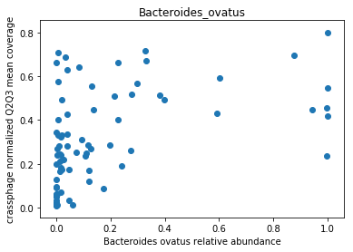
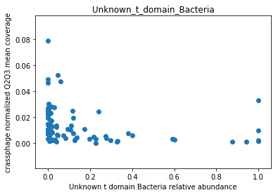
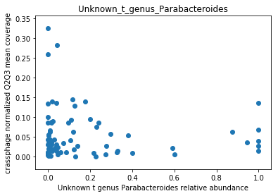
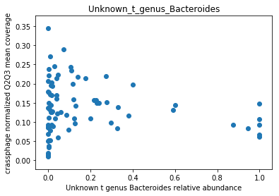
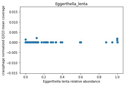
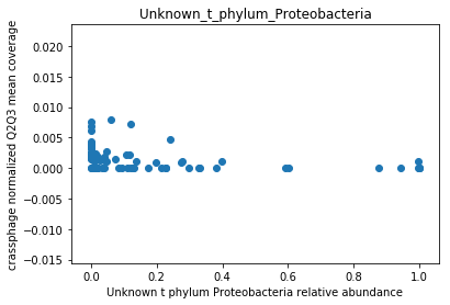
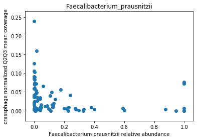
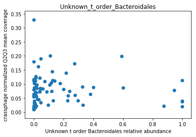
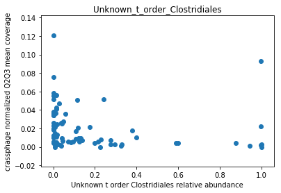
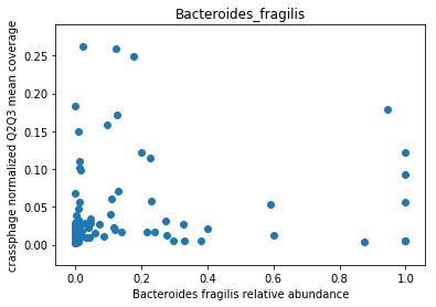
We can see that this list is dominated by members and close relatives of the Bacteroides genus, which is encouraging. In addition, a few other things are included, but we need to remember that in a regression model things that anti-correlate could also count as important features.
Exploring the mapping results with “gene mode”
We go back to anvi’o now, and dig a little bit more into the merged profile that we created using our snakemake.
Earlier, we used the interactive interface and saw the coverage and detection of “splits” across metagenomes. Our splits were approximately 20,000 nucleotide in size, and had no special biological significance. Now, we want to look at things in a higher resolution and with more biological significance, so we will look at the coverage and detection of genes across metagenomes. For that, we will use “gene mode”.
In order to use the anvi’o interactive interface in “gene mode”, we have to first create a collection. This is just a technical requirement, and we do this very easily by running this command:
anvi-script-add-default-collection -p PROFILE.db -c crAssphage-contigs.db
Now we can run the interactive interface in “gene mode”:
It might take a few minutes to load, because all the gene level statistics are calculated on-the-fly.
anvi-interactive -c crAssphage-contigs.db -p PROFILE.db --gene-mode -C DEFAULT -b EVERYTHING
Examining the mapping results in “gene mode”
Take some time to look at the results in the gene level. Do you see any interesting patterns?
Try to compare the results from one geographical location to the other, is there any difference?
Use right click on any gene (i.e. any radial portion of the figure), and click “inspect gene”, to look at single nucleotide variants (SNVs). Choose to inspect one gene that occurs in all samples (a “core” gene), and one gene that occurs in only some of the samples (an “accessory” gene). Do you see anything interesting in the SNV pattern?
The global distribution of phicrass001
Repeating the analysis with a different reference genome
It should now be easy to adapt our snakefile to work with a different reference genome. In fact, your snakefile shouldn’t include any details about the reference genome nor the locations of the bam files. These should be accepted as input from the user. To learn how to allow input from the user when running a snakefile, refere to the snakemake docummentation regarding the config file.
Now repeat the profiling this time with the bam files that correspond to phicrass, and the phicrass fasta file.
Once it is done, download the results to your local host, and use the interactive interface to examine the global distribution of phicrass001. How does it compare to the distribution of crassphage?
Try to examine the mapping results in “gene mode”, what can you say about the distribution of the phicrass genes?
Use the krakenHLL results to examine the distribution of the phicrass host Bacteroides intestinalis. How does it compare to the distribution of phicrass? and to that of crassphage?