

Table of Contents
- Introduction
- Parameters
- Case I: All I have is a bunch of FASTA files
- Case II: I want to work with my genome bins in anvi’o collections
- Case III: Case I + Case II (I want it all, because science)
- Accessing protein clusters
- Taking a quick look into a protein cluster
- Making selections on the display
- Highlighting certain protein clusters on the display
- Enriching the pangenomic display with additional information
This pangenomic workflow is for 2.0.2 and earlier versions of anvi’o. You can learn which version you have on your computer by typing anvi-profile --version in your terminal. The latest workflow and most up-to-date pangenomic is here, and comes with some significant improvements with respect to interactivity.
Cultivation of closely related microorganisms, and the subsequent recovery of their genomes, revealed that not all isolates share the same functional traits for a given population. On the other hand, individual isolates do not fully echo the functional complexity of naturally occurring microbial populations either. Large genomic collections is the only way to get closer to a more realistic picture of the pool of functions in a given clade of bacterial tree.
Overlapping and differing functions among the genomes of closely related organisms led to the introduction of a new concept, “pangenomics” (Tettelin et al., 2005), where genes across genomes are segregated into distinct groups: (1) the core-genome, (2) genes detected in multiple yet not in all genomes, and finally (3) isolate-specific genes that are detected only in a single genome. Pangenomic investigations are now widely used to dissect the functional traits of microorganisms, and to uncover environmentally- and clinically-important clusters of genes or functions.
Although multiple bioinformatics software are available to generate and/or visualize pangenomes, these solutions do not necessary offer flexible work environments, and hence limit the user’s ability to interact with their data.
This post describes the anvi’o workflow for pangenomics using a simple dataset. Using this workflow you can,
- Identify protein clusters,
- Visualize the distribution of protein clusters across your genomes,
- Organize genomes based on shared protein clusters,
- Interactively identify core, and core-like protein clusters,
- Extend analysis results with contextual information about your genomes,
- Compare MAGs from your projects with cultivar genomes from other sources.
You can use anvi’o for pangenomic analysis of your genomes even if you haven’t done any metagenomic work with anvi’o. All you need is an anvi’o installation and a FASTA file for each of your genomes.
Pangenomic workflow uses MCL, which is not a global dependency for anvi’o, hence you may not have it on your system even if you have anvi’o up and running. You can install it using this recipe.
Introduction
The program anvi-pan-genome is the main entry to the pangenomic workflow. Next chapters will demonstrate how it is used, but first, a brief understanding of what it does.
You can run anvi-pan-genome on external genomes, internal genomes, or using a mixture of the two. The difference between external and internal genomes in the context of anvi’o workflow is simple:
-
External genomes: Anything you have in a FASTA file format (i.e., a genome you downloaded from NCBI, or any other resource).
-
Internal genomes: Any genome bin you stored in an anvi’o collection (you can create an anvi’o collection by importing automatic binning results, or by using anvi’o to do human guided binning; if you would like to lear more about this please take a look at the metagenomic workflow).
File formats for external genome and internal genome descriptions differ slightly. This is an example --external-genomes file:
| name | contigs_db_path |
|---|---|
| Name_01 | /path/to/contigs-01.db |
| Name_02 | /path/to/contigs-02.db |
| Name_03 | /path/to/contigs-03.db |
| (…) | (…) |
The only thing you need is to define a name for your genome, and point the contigs_db_path for it (see the later chapters to see how can you get from you FASTA files to here).
The file format to describe internal genomes of interest is slightly more complex, but allows you to do quite a lot. Here is an example file for --internal-genomes:
| name | bin_id | collection_id | profile_db_path | contigs_db_path |
|---|---|---|---|---|
| Name_01 | Bin_id_01 | Collection_A | /path/to/profile.db | /path/to/contigs.db |
| Name_02 | Bin_id_02 | Collection_A | /path/to/profile.db | /path/to/contigs.db |
| Name_03 | Bin_id_03 | Collection_B | /path/to/another_profile.db | /path/to/another/contigs.db |
| (…) | (…) | (…) | (…) | (…) |
Any genome bin in any anvi’o collection can be included in the analysis (and you can combine these genome bins with cultivar genomes you have downloaded from elsewhere). Let’s talk about the parameters, and output files before we start with examples.
Parameters
When you run anvi-pan-genome with --external-genomes, or --internal-genomes, or both parameters, the program will
- Use DIAMOND (Buchnfink et al., 2015) in ‘fast’ mode (you can ask DIAMOND to be ‘sensitive’ by using the flag
--sensitive) by default to calculate similarities of each protein in every genome against every other protein (which clearly requires you to have DIAMOND installed). Alternatively you could use the flag--use-ncbi-blastto use NCBI’sblastpfor protein search.
A note from Meren: I strongly suggest you to do your analysis with the --use-ncbi-blast flag. Yes, DIAMOND is very fast, and it may take 8-9 hours to analyze 20-30 genomes with blastp. But dramatic increases in speed rarely comes without major trade-offs in sensitivity and accuracy, and some of my observations tell me that DIAMOND is not one of those rare instances. This clearly deserves a more elaborate discussion, and maybe I will have a chance to write it later, but for now take this as a friendly reminder.
-
Use every gene call, whether they are complete or not. Although this is not a big concern for complete genomes, metagenome-assembled genomes (MAGs) will have many incomplete gene calls at the end and at the beginning of contigs. They shouldn’t cause much issues, but if you want to exclude them, you can use the
--exclude-partial-gene-callsflag. -
Use the minbit heuristic that was originally implemented in ITEP (Benedict et al, 2014) to eliminate weak matches between two protein sequences (you see, the pangenomic workflow first identifies proteins that are somewhat similar by doing similarity searches, and then resolves clusters based on those similarities. In this scenario, weak similarities can connect protein clusters that should not be connected). Here is a definition of minbit: If you have two protein sequences
AandB, the minbit is defined asBITSCORE(A, B) / MIN(BITSCORE(A, A), BITSCORE(B, B)). Therefore, the minbit score of two sequences goes to1if they are very similar over their entire length, and it goes to0if they match over a very short stretch compared to their entire length (regardless of how similar they are at the aligned region), or their sequence identity is low. The default minbit is0.5, but you can change it using the parameter--minbit. -
Use the MCL algorithm (van Dongen and Abreu-Goodger, 2012) to identify clusters in protein similarity search results. We use
2as the MCL inflation parameter by default. This parameter defines the sensitivity of the algorithm during the identification of the protein clusters. More sensitivity means more clusters, but of course more clusters does not mean better inference of evolutionary relationships. More information on this parameter and it’s effect on cluster granularity is here http://micans.org/mcl/man/mclfaq.html#faq7.2, but clearly, we, the metagenomics people will need to talk much more about this. -
Utilize every protein cluster, even if they occur in only one genome in your analyses. Of course, the importance of singletons or doubletons will depend on the number of genomes in your analysis, or the question you have in mind. However, if you would like to define a cut-off, you can use the parameter
--min-occurrence, which is 1, by default. Increasing this cut-off will improve the clustering speed and make the visualization much more manageable, but again, this parameter should be considered in the context of each study. -
Use only one CPU. If you have multiple cores, you should consider increasing that number using the
--num-threadsparameter. The more threads, the merrier the time required for computation. -
Utilze previous search results if there is already a directory. This way you can play with the
--minbit,--mcl-inflation, or--min-occurrenceparameters without having to re-do the protein search. However, if you have changed the input protein sequences, either you need to remove the output directory, or use the--overwrite-output-destinationsflag to redo the search.
You need another parameter? Well, of course you do! Let us know, and let’s have a discussion. We love parameters.
Once anvi-pan-genome is done, it will generate an output directory that will be called pan-output by default (and you should change it to a more meaningful one using the --output-dir parameter). This directory will include essential files such as search results and protein clusters, and another special directory with all the necessary files to invoke an anvi’o interactive interface using this command:
anvi-interactive -s samples.db -p profile.db -t tree.txt -d view_data.txt -A additional_view_data.txt --manual --title "My Pangenome"Let’s see some examples.
Case I: All I have is a bunch of FASTA files
Assume you have three FASTA files for three E. coli strains you want to analyze with anvi-pan-genome (you can download these genomes and play with them if you click those links):
Let’s assume you downloaded each one of them, and now your work directory looks like this:
$ ls -l
-rw-r--r--   1 meren  staff  1362351 Jun 29 14:42 E_coli_BL21.fa.gz
-rw-r--r--   1 meren  staff  1383249 Jun 29 14:43 E_coli_B_REL606.fa.gz
-rw-r--r--   1 meren  staff  1604922 Jun 29 14:43 E_coli_O111.fa.gz
The first thing is to generate an anvi’o contigs database for each one of them, and run HMMs on them to identify bacterial single-copy core genes. Here is an example for one genome:
$ gzip -d E_coli_BL21.fa.gz
$ anvi-gen-contigs-database -f E_coli_BL21.fa -o E_coli_BL21.db --split-length -1
$ anvi-run-hmms -c E_coli_BL21.db
If you haven’t created an anvi’o contigs database before, please read this section from the metagenomics tutorial to learn the details of this step.
Doing the same thing above for all genomes in a serial manner would have looked like this, in case you are a work-in-progress BASH scripting guru:
for g in E_coli_BL21 E_coli_B_REL606 E_coli_O111
do
    gzip -d $g.fa.gz
    anvi-gen-contigs-database -f $g.fa -o $g.db -L -1
    anvi-run-hmms -c $g.db
done
At the end of this, my directory looks like this:
-rw-r--r--  1 meren  staff  6778880 Jun 29 14:52 E_coli_BL21.db
-rw-r--r--  1 meren  staff  4624090 Jun 29 14:45 E_coli_BL21.fa
-rw-r--r--  1 meren  staff  4567241 Jun 29 14:46 E_coli_BL21.h5
-rw-r--r--  1 meren  staff  6904832 Jun 29 14:52 E_coli_B_REL606.db
-rw-r--r--  1 meren  staff  4695964 Jun 29 14:46 E_coli_B_REL606.fa
-rw-r--r--  1 meren  staff  4638100 Jun 29 14:48 E_coli_B_REL606.h5
-rw-r--r--  1 meren  staff  7996416 Jun 29 14:53 E_coli_O111.db
-rw-r--r--  1 meren  staff  5447818 Jun 29 14:48 E_coli_O111.fa
-rw-r--r--  1 meren  staff  5379365 Jun 29 14:49 E_coli_O111.h5
Now all anvi’o contigs databases are ready, it is time to prepare the --external-genomes file:
| name | contigs_db_path |
|---|---|
| BL21 | E-coli-BL21.db |
| B_REL606 | E-coli-B_REL606.db |
| O111 | E-coli-O111.db |
And run anvi-pan-genome:
$ anvi-pan-genome --external external_genomes.txt -o pan-output --num-threads 20At the end of this, I can run the anvi-interactive to see my results:
$ cd pan-output/pan-output
$ anvi-interactive -s samples.db -p profile.db -t tree.txt -d view_data.txt -A additional_view_data.txt --manual --title "Pangenome of three E. coli's"
If you click Draw, you will get a pangenomic display. But if you do it after selecting protein_clusters from the Samples > Sample order menu, this time you will get a display of your pangenome along with the organization of your genomes based on protein clusters they share (see the tiny tree on the right side):
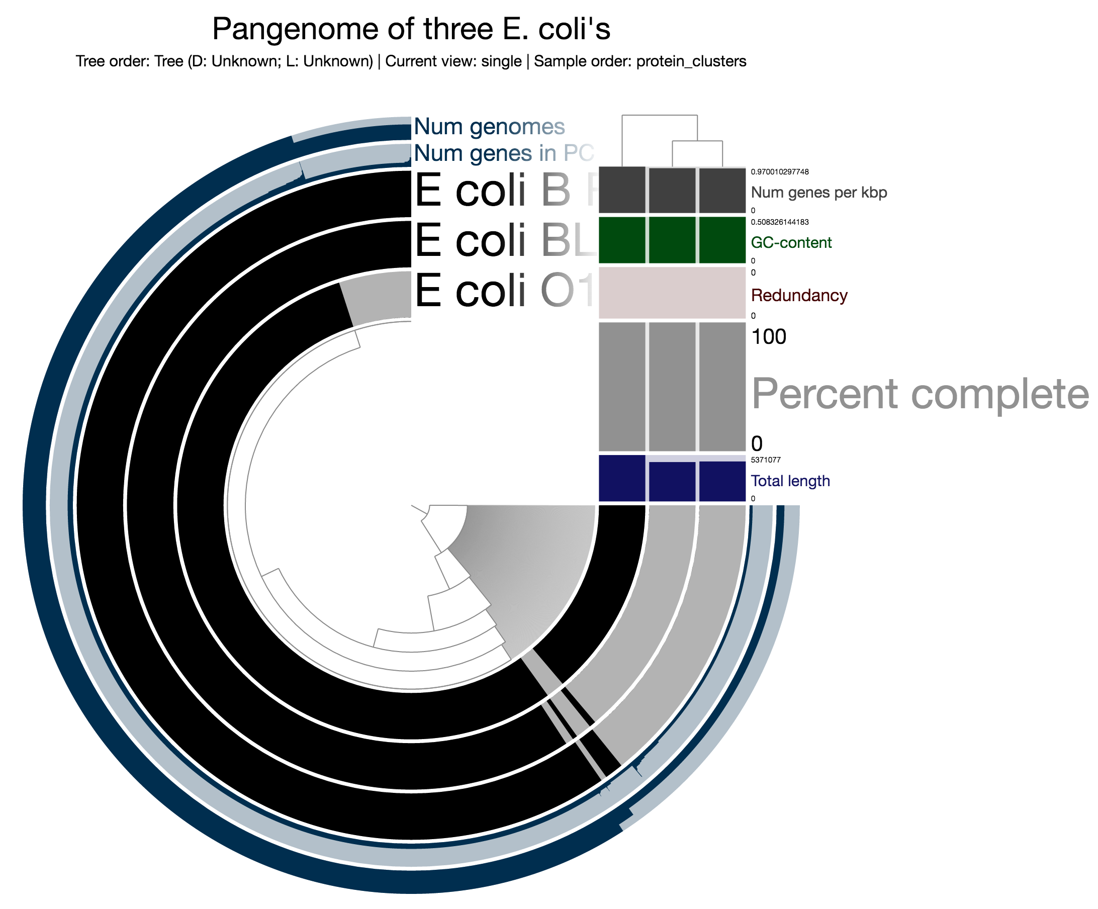
Alright. This doesn’t look quite fancy. But let’s hope your actual genomes will look be much more informative and interesting than three random E. coli’s. To find out ways to enrich your display by including more information about your genomes, continue reading.
Case II: I want to work with my genome bins in anvi’o collections
If you have been doing your metagenomic analyses using anvi’o, it is much more easier to run the pangenomic workflow. All you need to do is to create a --internal-genomes file like this one,
| name | bin_id | collection_id | profile_db_path | contigs_db_path |
|---|---|---|---|---|
| MAG_01 | DWH_SAND_Bin_01 | SAND | DWH-SAND-MERGED/PROFILE.db | SAND-CONTIGS.db |
| MAG_02 | DWH_SAND_Bin_04 | SAND | DWH-SAND-MERGED/PROFILE.db | SAND-CONTIGS.db |
| MAG_03 | SML_SEWAGE_Bin_08 | SEWAGE | SML-SEWAGE-MERGED/PROFILE.db | SEWAGE-CONTIGS.db |
And run anvi-pan-genome using it instead:
$ anvi-pan-genome --internal internal_genomes.txt -o pan-output --num-threads 20The rest is the same!
Case III: Case I + Case II (I want it all, because science)
You are lucky! Just mix your internal and external genomes in the same command line:
$ anvi-pan-genome --internal internal_genomes.txt --external external_genomes.txt -o pan-output --num-threads 20Accessing protein clusters
We are currently planning to advance pangenomic workflow in anvi’o with improved interactivity and integrated functionality to query data. We will continue to update this post as we progress. For now please bear with us as we explain some not-so-elegant ways to take care of certain things. For instance, we added this section after Alex asked about this (see the comment section below). If you need help getting things done, please just ask!
Every protein cluster in your analysis results contains one or more gene calls that originate from one or more genomes. It is also common to find protein clusters that contain more than one gene call from a single genome is also common (i.e., all multi-copy genes in a given genome will end up in the same protein cluster).
Sooner or later you will start getting curious about some of the protein clusters, and want to learn more about them.
Taking a quick look into a protein cluster
One of the key output files to investigate the protein clusters you see in the pangenomic display is the file protein-clusters.txt, which looks like this:
| entry_id | gene_caller_id | protein_cluster_id | genome_name | sequence |
|---|---|---|---|---|
| 0 | 3685 | PC_00001990 | E_coli_BL21 | MATTQQSGFAPAASPLASTIVQTPDDAIVAGFTSIPSQ(…) |
| 1 | 3735 | PC_00001990 | E_coli_B_REL606 | MATTQQSGFAPAASPLASTIVQTPDDAIVAGFTSI(…) |
| 2 | 4590 | PC_00001990 | E_coli_O111 | MATTQQSGFAPAASPLASTIVQTPDDAIVAGFTSIPSQGD(…) |
| 3 | 3076 | PC_00001859 | E_coli_BL21 | MKPIFSRGPSLQIRLILAVLVALGIIIADSRLGTFSQIR(…) |
| 4 | 3126 | PC_00001859 | E_coli_B_REL606 | MKPIFSRGPSLQIRLILAVLVALGIIIADSRLGTFSQ(…) |
| 5 | 3998 | PC_00001859 | E_coli_O111 | MKPIFSRGPSLQIRLILAVLVALGIIIADSRLGTFSQIRT(…) |
| 6 | 763 | PC_00001992 | E_coli_BL21 | MAETKIVVGPQPFSVGEEYPWLAERDEDGAVVTFTGKVRN(…) |
| 7 | 756 | PC_00001992 | E_coli_B_REL606 | MAETKIVVGPQPFSVGEEYPWLAERDEDGAVVTFT(…) |
| 8 | 832 | PC_00001992 | E_coli_O111 | MAETKIVVGPQPFSVGEEYPWLAERDEDGAVVTFTGKVRN(…) |
| (…) | (…) | (…) | (…) | (…) |
As you probably already know, the Mouse tab in the interactive interface allows you to see the information underneath your cursor while you brows the interactive interface. If you are curious to know a bit more about a given protein cluster, you can go back to your terminal and use grep:
$ grep 'PC_00000914' ../protein-clusters.txt
13544	2554	PC_00000914	E_coli_BL21	MCIGVPGQIRTIDGNQAKVDVCGIQRDVDLTLVGSCDEN(...)
13545	2592	PC_00000914	E_coli_B_REL606	MCIGVPGQIRTIDGNQAKVDVCGIQRDVDLTLVGSCDEN(...)
13546	3378	PC_00000914	E_coli_O111	MCIGVPGQIRTIDGNQAKVDVCGIQRDVDLTLVGSCDEN(...)
Making selections on the display
Alternatively, you may want to focus on groups of protein clusters. Using the anvi’o interactive interface you can bin your protein clusters, and store them as collections to process them further.
Just as an example let’s assume you are interested in gene calls that are unique to the E. coli genome O111 in our mock analysis on this page. You can select all protein clusters the following way:
And then you can store them as a collection. Let’s assume you clicked Bins > Store bin collection, and typed in PCs in the input box as a collection name, and finally clicked Store to create a collection (clearly you can choose any name as far as you promise you will later remember it later). Now you can go back to the terminal, and export bins in the PCs collection (we have only one bin this time, but of course there is no limit how many bins you select):
In order to use the following program, you must have the latest version of the repository from the master. But if you are using anvi’o v2.0.2, and really want to be able to use this functionality without with installing a new version from the repository, send Meren an e-mail via meren at uchicago, and you will get a recipe for a workaround.
$ anvi-script-PCs-to-gene-calls ../protein-clusters.txt -p profile.db -C PCs
Collection "PCs" .............................: 1 protein cluster bins describes 946 PCs.
Protein clusters .............................: 13,775 entries are read into the memory.
Genomes found (3) ............................: E_coli_BL21, E_coli_B_REL606, E_coli_O111.

* Storing gene caller ids:

Gene calls (0) [E_coli_BL21/Bin_1] ...........: gene-caller-ids_for-PCs-E_coli_BL21-Bin_1.txt
Gene calls (0) [E_coli_B_REL606/Bin_1] .......: gene-caller-ids_for-PCs-E_coli_B_REL606-Bin_1.txt
Gene calls (1,251) [E_coli_O111/Bin_1] .......: gene-caller-ids_for-PCs-E_coli_O111-Bin_1.txt
OK. Each of these three files that are just created in your work directory contains gene caller ids for protein clusters matching the red selection for each genome. Expectedly, there are 0 calls for E_coli_BL21 and E_coli_B_REL606, since the protein clusters in that particular selection are unique to E_coli_O111.
Since we have a handle on the gene calls for the given section of the pangenome, we can export gene sequences for the gene calls using the anvi’o contigs database for E_coli_O111:
$ anvi-get-dna-sequences-for-gene-calls -c ../../E_coli_O111.db \
                                        --gene-caller-ids gene-caller-ids_for-PCs-E_coli_O111-Bin_1.txt \
                                        -o gene-caller-ids_for-PCs-E_coli_O111-Bin_1.fa
Resulting FASTA file will have sequences that are unique to E_coli_O111 genome:
$ head -n 100 gene-caller-ids_for-PCs-E_coli_O111-Bin_1.fa
>259|contig:260866153|start:294792|stop:297237|direction:r|rev_compd:True|length:2445
ATGCCAACACCAACCATCATCAAAACACTCGCCACCCACCGCGAAAAACCGTTTGTCAGCGTCGTCACGCCAACCTGGAACCGCGGCGCATTCCTGCCGTACCTGCTCTATATGTACCGC
TATCAGGATTACCCGGCAGACCGCCGCGAACTCATCATCCTCGACGATTCCCCACAAAGCCATCAACACATCATCGACCGCCTGACCAATGGCACGCCGGAAGCCTTTAACATCCGCTAC
ATCCATCACCCGGAAAAACTGCCGCTGGGCAAAAAACGCAACATGCTCAACGAACTGGCGCGCGGCGAATACATCCTCTGCATGGATGATGACGACTACTATCCGGCAGATAAAATCTCT
(...)
>3514|contig:260866153|start:3563822|stop:3564260|direction:f|rev_compd:False|length:438
ATGAAGCCACGAAATATTAATAATAGCCTACCACTGCAACCATTAGTTCCTGATCAGGAGAACAAAAATAAGAAAAATGAAGAGAAATCCGTTAATCCAGTTAAAATCACAATGGGGTCT
GGTTTAAATTATATTGAACAAGAATCTCTTGGAGGAAAATATCTAACACATGATTTGTCAATAAAGATAGCGGATATTTCTGAAGAGATAATTCAGCAAGCAATATTATCTGCTATGAGC
ATATATAAATTTTCGATAACAGATGATTTAATGAGTATGGCTGTAAATGAACTCATAAAACTGACCAAAATAGAGAATAATGTAGACCTGAATAAATTCACTACTATATGCACAGACGTT
(...)
>3675|contig:260866153|start:3728029|stop:3730837|direction:r|rev_compd:True|length:2808
ATGATTACTCATGGTTTTTATGCCCGGACCCGGCACAAGCATAAGCTAAAAAAAACATTTATTATGCTTAGCGCTGGTTTAGGATTGTTTTTTTATGTTAACCAGAACTCATTTGCAAAC
GGTGAAAATTATTTTAAATTGAGTTCAGATTCAAAACTGTTAACTCAAAATGTTGCTCAGGATCGCCTTTTTTATACGTTGAAAACAGGTGAAACTGTTTCCAGTATTTCTAAATCACAA
GGTATCAGTTTATCCGTAATTTGGTCACTGAATAAACATTTATACAGTTCCGAAAGCGAAATGCTGAAGGCTGCGCCTGGCCAGCAGATCATTTTGCCACTCAAAAAACTGTCTGTTGAA
(...)
>5104|contig:260866153|start:5263671|stop:5264277|direction:r|rev_compd:True|length:606
ATGATTAAAAATGACAAGGCATGGATAGGAGACTTGCTGGGCGGGCCGCTCATGAGCAGGGAAAGCCGCGTCATTGCCGAGCTGTTGCTAACCGATCCCGATGAACAGACATGGCAAGAG
CAAATTGTTGGCCACAACATTTTACAAGCCTCTTCTCCTAATACCGCAAAACGTTACGCGGCAACAATCAGGCTTCGCCTGAACACGCTTGATAAAAGCGCGTGGACATTAATTGCCGAA
GGTAGCGAGCGGGAACGCCAGCAACTTCTGTTTGTGGCTCTGACGCTACATTCGCCGGTAGTTAAGGATTTTCTGGCTGAAGTGGTGAACGATCTGCGCAGGCAGTTCAAGGAAAAGTTG
(...)
>2606|contig:260866153|start:2621068|stop:2622004|direction:r|rev_compd:True|length:936
GTGAATAGTATAGCAATTTTAGAAGCAGTGAACACCTCTTATGTACCATTCAACGGTCAGCAAATTATCACCGCCATGGCTGCCGGAGTTGCATATGTTGCGATGAAGCCAATCGTTGAA
AACCTTGGAATGAGCTGGTCAACGCAGCAAACAAAACTCATGAAGCAGATTAGCAAATTCAACTGTGTTCATATGAACATGGTTGCCGCTGATGGGAAGCTTCGTAAGCTACTCTGCCTT
CCTTTGAAGAAGTTAAATGGATGGCTGTTCAGCATCAACCCTGAGAAAGTTCGTGCTGACATCCGTGATAAACTGATTCAGTACCAGGAAGAATGCTTTAGCGTGCTGCATGACTACTGG
(...)
>1585|contig:260866153|start:1632818|stop:1633127|direction:f|rev_compd:False|length:309
ATGGGGAGAGCCGACTGGCGCGCCATGCTTGCCGGGATGACATCCACCGAATATGCCGACTGGCGACGTTTTTACTGCACGCATTATTTTCAGGATACCCAGCTGGATATGCATTTTTCC
GGGCTGATGTACGCCGTACTCAGCCTGTTTTTTTGCGATCCGGATATGCATCCGGCGGATTTCAGCCTGTTCGCTCCGGAGGCAGAGGAAGGACAGGCGGAGACGCCGGACGAAAATGAT
GTACTGATGCAGAAGGCGGCGGGCCTCGCCGGTGGAGTCCGTTTCGGGGAGGAGGGAAGGAGGTTGTGA
>264|contig:260866153|start:300090|stop:300426|direction:f|rev_compd:False|length:336
ATGGGGATCAGTTTTCAGCAGGCATTGGGAGTACATCCGCAGGCAGTGAAGTTACGTCTTGAGAGGACCGAGCTACTGACTGCGAATCTGGCGAACGTCGATACGCCAAATTTCAAGGCT
AAAGATATTGATTTTGCCAGGGAGATGCAACGGGCAAATAACGCGGCGGTGGATGTCCAGTACCGCGTGCCGATGCAGCCGTCGGAAGATGGCAACACCGTGGAACTGAACAGCGAGCAG
GCGCGGTTTTCACAAAATAGTATGGATTATCAAAGCAGTTTGACCTTTCTGAATCTGCAAATCAGCGGCATCAGAGAGGCCATTGAAGGGAAATAA
>2462|contig:260866153|start:2499185|stop:2499857|direction:f|rev_compd:False|length:672
ATGTGTGGACGCTTTGCCCAATCCCAAACGCGTGAAGATTACCTTGCGCTTCTCGCGGAAGATATTGAACGCGATATTCCCTACGATCCCGAACCCATTGGCAGATACAACGTCGCGCCG
GGAACCAAAGTTCTTCTGCTCAGTGAACGTGATGAACACCTTCATCTGGATCCGGTTTTCTGGGGATATGCTCCCGGATGGTGGGATAAACCGCCGCTGATTAACGCCCGCGTAGAAACT
GCGGCCACCAGTCGTATGTTTAAACCGCTCTGGCAACATGGTCGGGCAATCTGTTTTGCCGATGGCTGGTTTGAGTGGAAAAAAGAAGGCGACAAAAAACAGCCTTATTTTATCTATCGC
(...)
>2469|contig:260866153|start:2506868|stop:2507864|direction:f|rev_compd:False|length:996
ATGAGTAACCTGACAGGCACCGATAAAAGCGTCATCCTGCTGATGACCATTGGCGAAGACCGGGCGGCAGAGGTGTTCAAGCACCTCTCCCAGCGCGAAGTGCAAACCCTGAGCGCTGCA
ATGGCGAACGTCACGCAGATCTCCAACAAGCAGCTAACCGATGTGCTGGCGGAGTTTGAGCAAGAAGCTGAACAGTTTGCCGCACTGAATATCAACGCCAACGATTATCTGCGTTCGGTA
TTGGTCAAAGCTCTGGGTGAGGAACGTGCCGCCAGCCTGCTGGAAGATATTCTCGAAACTCGCGATACCGCCAGCGGTATTGAAACGCTCAACTTTATGGAGCCGCAGAGCGCCGCCGAT
(...)
>2470|contig:260866153|start:2507856|stop:2508543|direction:f|rev_compd:False|length:687
ATGTCTGATAATCTGCCGTGGAAAACCTGGACGCCGGACGATCTCGCGCCACCACAGGCAGAGTTTGTGCCCATGGTCGAGCCGGAAGAAACCATCATTGAAGAGGCCGAACCCAGCCTT
GAGCAGCAACTGGCGCAACTGCAAATGCAGGCCCATGAGCAAGGTTATCAGGCGGGGATTGCCGAAGGTCGCCAGCAAGGTCATGAGCAGGGCTATCAGGAAGGACTGGCCCAGGGGCTG
GAGCAAGGTCTGGCAGAGGCGAAGTCTCAACAAGCGCCAATTCATGCCCGGATGCAGCAACTGGTCAGCGAATTTCAAACTACCCTTGATGCACTTGATAGTGTGATTGCTTCGCGCCTG
(...)
Highlighting certain protein clusters on the display
In order to use the following program, you must have the latest version of the repository from the master. But if you are using anvi’o v2.0.2, and really want to be able to use this functionality without with installing a new version from the repository, send Meren an e-mail via meren at uchicago, and you will get a recipe for a workaround.
It is also possible to show a particular group of protein clusters in the pangenomic display. If you have a list of protein clusters, you can import them into the profile database as a collection. To demonstrate it using the mock example, let’s assume what you want to do is to identify protein clusters that contain at least one gene, translated amino acid sequence of which has more than 500 residues. This awk one-liner will give me a TAB-delimited file that can be used to import into the profile database using anvi-import-collection:
$ awk '{if (length($5) > 500) print $3 "\t LONG_PCs"}' ../protein-clusters.txt \
		| uniq > test-collection.txt
Although in this case there is only one bin, LONG_PCs, of course you may have as many as you want for a real-world application. If you import this file into the profile database as a collection the following way,
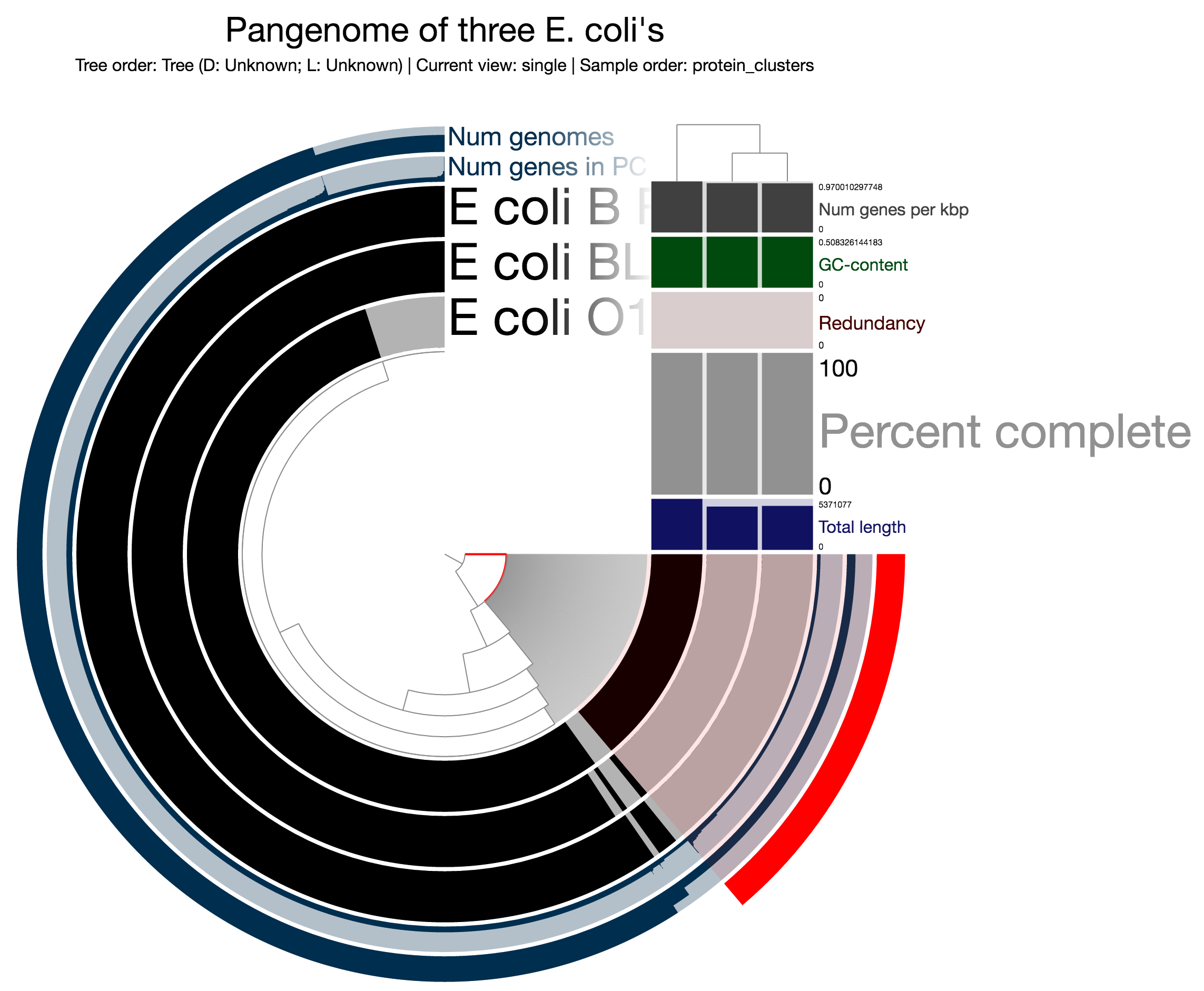
$ anvi-import-collection test-collection.txt -p profile.db -C LONG_PCsThis is what you should see after running the interactive interface again, and loading the collection LONG_PCs:
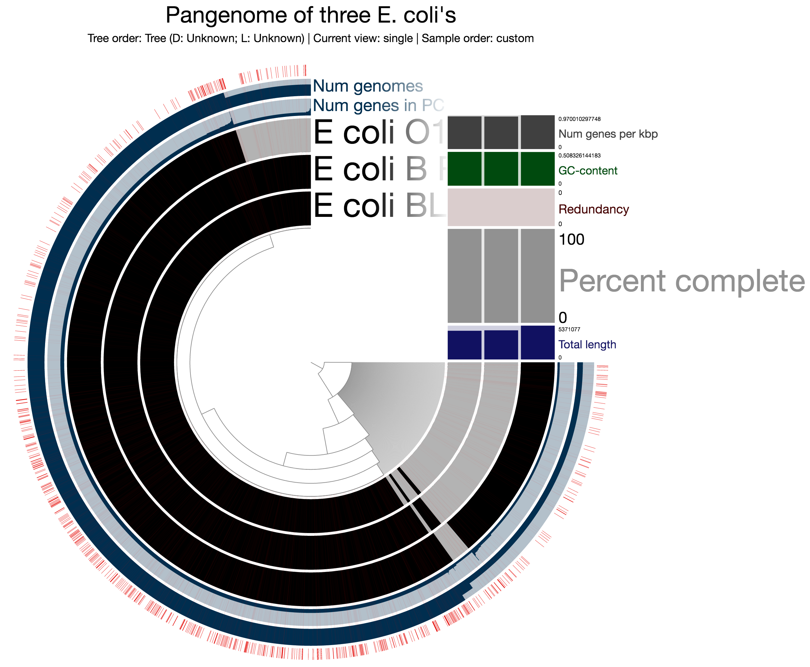
Interesting! The proportion of the longer genes vs. shorter ones seem to be much higher for the core, compared to the what is specific to E_coli_O111 (Meren: when I was coming up with this example I didn’t expect to see this, now I wonder if it is a methodological artifact or a biologically relevant or expected outcome).
Of course adding new collections to the profile database is not the only way to highlight PCs of interest on the display. You can add as many columns as you like to the file additional_view_data.txt.
Enriching the pangenomic display with additional information
The output directory of a pangenomic analysis will contain two files, additional_view_data.txt and anvio_samples_info.txt, both of which will contain some default information about genomes and PCs. You can certainly add more contextual information about your genomes to increase the number of layers by adding more columns to the additional_view_data.txt, and re-generating the samples.db after adding more columns to the anvio_samples_info.txt file.
For instance, here is a slightly richer analysis of 30 genomes:
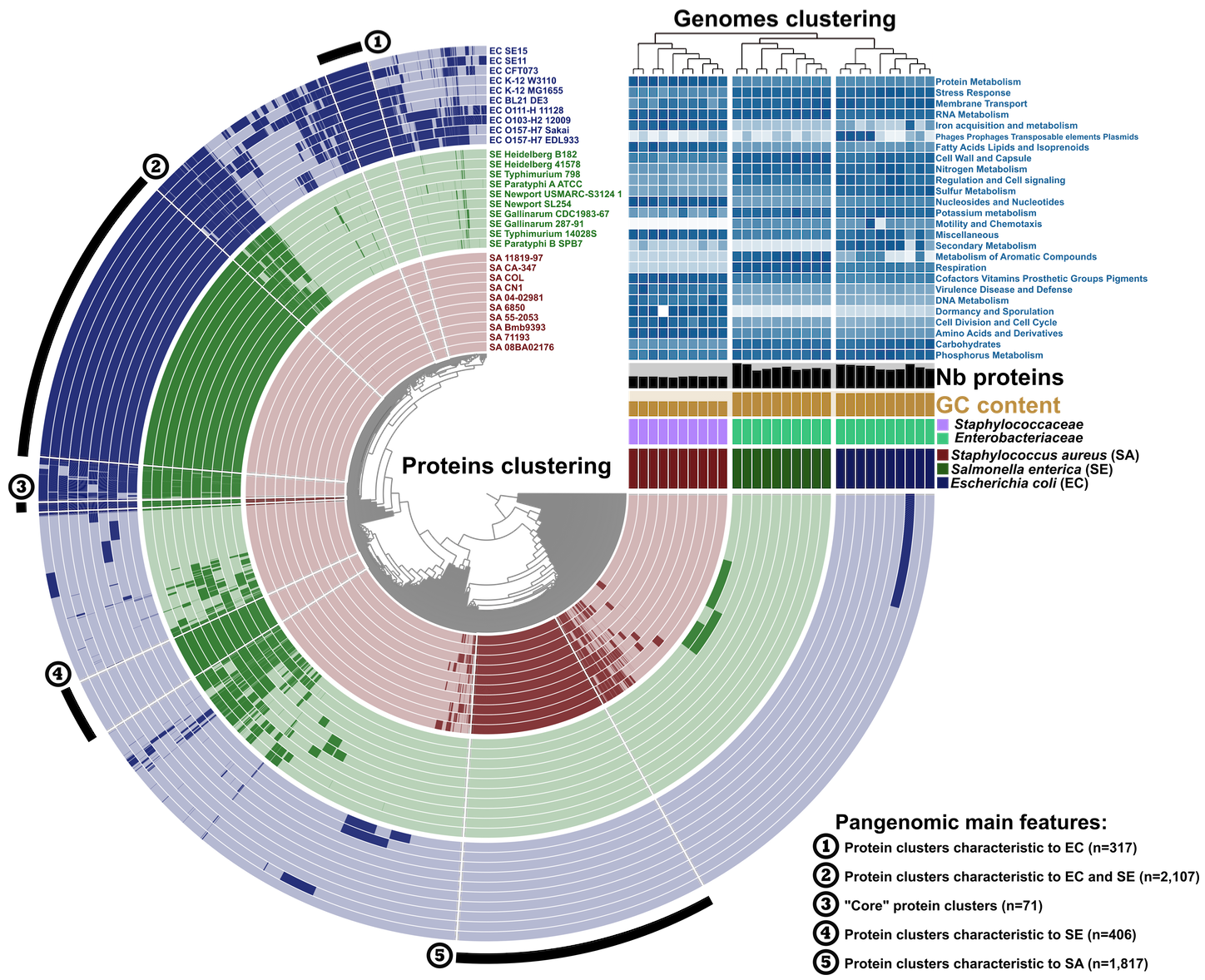
The rest is up to your inner artist.