Materials from an anvi'o workshop at the Microbiome Center


Table of Contents
- The Microbiome Center Metagenomics Workshop
- A bit of setup
- Saving number of threads as an environment variable
- Loading the anvi’o environment
- Download some databases
- Part I: Getting started with anvi’o (20 min.)
- Going from a MAG FASTA file to a contigs-db (7 min.)
- Annotating SCGs in the MAG (4 min.)
- Checking the taxonomy of the MAG (4 min.)
- Estimating MAG completeness (5 min.)
- Part II: Explore the ecology of bacterial populations from an FMT donor across FMT recipients (7 min.)
- Prepare fasta reference
- Map metagenomes against reference (~4 min)
- Profile the mapping results with anvi’o (~3 min)
- Visualize mapping results with anvi’o
- Part III: Investigating metabolism in MAGs (15 min)
- Annotate genes in the MAG with KEGG KOfams (~5 min)
- Estimating metabolism (~3 min)
- Visualizing a heatmap of metabolic completeness across MAGs (~5 min)
- Computing enrichment of metabolic pathways in groups of genomes (~2 min)
- Takeaways

In February 2022, the Microbiome Center and Duchossois Family Institute at the University of Chicago hosted a metagenomics and metabolomics workshop, featuring anvi’o for the metagenomics part. Below, you’ll find a copy of our workshop materials, so you can follow along even if you missed this event.
You’ll learn about some anvi’o basics like how to work with anvi’o databases, how to annotate genes, and how to estimate genome completeness and taxonomy. Then, you’ll do some read recruitment and visualize the results in the interactive interface. Finally, you’ll practice estimating metabolism from gene annotations.
Matt Schechter and Iva Veseli taught this workshop with the help of the fearless Matthew Klein, who graciously served as teaching assistant. Feel free to reach out to any of them if you have questions about the materials. You can find their contact info on this page, or you can send them a message on the anvi’o Discord server:

The Microbiome Center Metagenomics Workshop
In this workshop, you will be learning how to perform a variety of genomic and metagenomic analyses using the software platform anvi’o. As you follow along with the workshop, you can use this document to reference some of the key commands we use. Also, you can look back at this file afterwards to remember what we worked on and how we did each step.
Background on the data
We will be using Fecal Matter Transplant (FMT) data from Watson et al., 2021 where they investigated which microbes from donors successfully colonized in recipients, and identified microbial genomic features that are predictive of successful colonization. This was explored by performing shotgun metagenomic sequencing on stool samples from donors and recipients at different time points. Today, we will be using a subset of Metagenome Assembled Genomes (MAGs) that were assembled from the donor data. We will learn how to detect these genomes in recipient metagenomes. Additionally, we will explore methods for determining the taxonomy and metabolic potential of these MAGs. We will not be discussing metagenomic binning below, so if you need to catch up on how MAGs are created from metagenomic data check out this post with an applied example: Chapter I: Genome-resolved Metagenomics.
Background on anvi’o
The software we will be using today to learn metagenomics is anvi’o.
anvi’o (analysis and visualization of ‘omics data) is an open source software platform that has a strong support community for empowering biologists and developing new tools to get the most out of microbial ‘omics data (metagenomics, transcriptomics, genomics, etc.). There are a ton of features and extensive documentation regarding its capabilities but we will quickly mention 4 key points that make anvi’o a catalyst for computational microbiology.
- Integrated and interactive ‘omics analyses: anvi’o allows you to interactively work with your data using the interactive interface. This allows you to probe the finest details of your data by inspecting coverage plots, viewing single-nucleotide variants, BLASTing sequences of interest, organizing complex metagenomic data into informative figures, and more. We will be exploring this live in the workshop.
- Snakemake workflows for high-throughput analyses: anvi’o has leveraged the workflow software called Snakemake to automate key steps in ‘omics analyses. This allows you to analyze a lot of data simultaneously! Anvi’o workflows come with a configuration file that allows you to customize the workflow to your scientific needs. Some popular anvi’o workflows are the metagenomics workflow and the pangenomics workflow.
- Consolidated data structures: anvi’o has powerful data integration objects, such as a contigs database (contigs-db) and profile database (profile-db), that combine all kinds of genomic data together to keep things organized. (Ever used Snapgene? The
.DNAfile that’s created after you make a change on a plasmid map is an analogous idea — except that it is a proprietary format that can only be opened with Snapgene, while anvi’o databases are SQL-based and can be queried outside of anvi’o programs.)- Specifically, the contigs-db stores all kinds of information that can be extracted from a fasta file such as: gene calls, annotations, taxonomy, and sequence statistics.
- The profile-db. This object stores information regarding read-recruitment data including: coverage, detection, single-nucleotide variance, single amino acid variance, etc.
- We will be using both contigs-dbs and profile-dbs in the tutorial below so please use the hyperlinks above to explore more!
- Large user community and under active development: anvi’o is community driven! Whether you need technical help or non-technical help, anvi’o has multiple ways to ask questions about your science and connect with other scientists.
Anvi’o is not the only software for ‘omics work out there. We consider it one of the most comprehensive (though we are certainly biased :), but you can always look for other options if you’d prefer. Most analyses that will be discussed in the workshop are general metagenomics concepts that could be implemented in other tools.
A bit of setup
Before we begin, please confirm you can correctly copy/paste the commands in the code blocks into your terminal. We recommend you have a text editor open where you can copy/paste the commands below so you can edit/modify the commands them before you run them on the command line.
Open your Terminal (if using OSX / Linux) or WSL (Ubuntu) prompt (if using Windows Subsystem for Linux) and use the cd command to navigate to the folder where you want to store the workshop datapack and run analyses. Use the following commands to 1) download the datapack DFI_ANVIO_WORKSHOP.tar.gz into your current folder, and 2) unpack the datapack and navigate into that directory:
# 1) download the datapack from the internet (specifically the University of Oldenburg cloud)
curl -L https://cloud.uol.de/public.php/dav/files/cTGMSJ7HZ3b2PoC \
     -o DFI_ANVIO_WORKSHOP.tar.gz

# 2) unpack data and move into the datapack folder
tar -zxvf DFI_ANVIO_WORKSHOP.tar.gz && cd DFI_ANVIO_WORKSHOP
Get familiar with the contents of this datapack by running the ls command. If your output does not look the same as below then you are in the wrong directory of your computer!
$ ls
01_FASTA                           FMT_LOW_FITNESS_KC_MAG_00082.db
FMT_HIG_FITNESS_KC_MAG_00022.db    FMT_LOW_FITNESS_KC_MAG_00082.fasta
FMT_HIG_FITNESS_KC_MAG_00022.fasta FMT_LOW_FITNESS_KC_MAG_00091.db
FMT_HIG_FITNESS_KC_MAG_00051.db    FMT_LOW_FITNESS_KC_MAG_00091.fasta
FMT_HIG_FITNESS_KC_MAG_00051.fasta FMT_LOW_FITNESS_KC_MAG_00097.db
FMT_HIG_FITNESS_KC_MAG_00055.db    FMT_LOW_FITNESS_KC_MAG_00097.fasta
FMT_HIG_FITNESS_KC_MAG_00055.fasta FMT_LOW_FITNESS_KC_MAG_00099.db
FMT_HIG_FITNESS_KC_MAG_00116.db    FMT_LOW_FITNESS_KC_MAG_00099.fasta
FMT_HIG_FITNESS_KC_MAG_00116.fasta FMT_LOW_FITNESS_KC_MAG_00100.db
FMT_HIG_FITNESS_KC_MAG_00120.fasta FMT_LOW_FITNESS_KC_MAG_00100.fasta
FMT_HIG_FITNESS_KC_MAG_00145.db    FMT_LOW_FITNESS_KC_MAG_00106.db
FMT_HIG_FITNESS_KC_MAG_00145.fasta FMT_LOW_FITNESS_KC_MAG_00106.fasta
FMT_HIG_FITNESS_KC_MAG_00147.db    FMT_LOW_FITNESS_KC_MAG_00118.db
FMT_HIG_FITNESS_KC_MAG_00147.fasta FMT_LOW_FITNESS_KC_MAG_00118.fasta
FMT_HIG_FITNESS_KC_MAG_00151.db    FMT_LOW_FITNESS_KC_MAG_00129.db
FMT_HIG_FITNESS_KC_MAG_00151.fasta FMT_LOW_FITNESS_KC_MAG_00129.fasta
FMT_HIG_FITNESS_KC_MAG_00162.db    FMT_LOW_FITNESS_KC_MAG_00130.db
FMT_HIG_FITNESS_KC_MAG_00162.fasta FMT_LOW_FITNESS_KC_MAG_00130.fasta
FMT_HIG_FITNESS_KC_MAG_00178.db    MAG_metadata.txt
FMT_HIG_FITNESS_KC_MAG_00178.fasta backup_data
FMT_LOW_FITNESS_KC_MAG_00079.db    big_data
FMT_LOW_FITNESS_KC_MAG_00079.fasta profile_mean_coverage.db
We will explain what these files are below, but one special thing to remember is that the backup_data/ folder contains the results and intermediate files that we will be generating throughout the workshop. If for some reason you have problems running certain programs, check that directory for the output of each step so you can continue on with the tutorial.
Saving number of threads as an environment variable
Many of the programs we will run are multi-threaded. We will create an environment variable storing the number of threads to use. Most laptops today have at least four cores, so we suggest setting the number of threads to 4:
THREADS=4
NOTE: If you have fewer than 4 cores you will want to set this number lower to avoid overworking your system and slowing everything down.
In the commands throughout this file, you will see that we use $THREADS to access this variable. You can always replace that with an actual integer if you prefer to set the number of threads yourself (but using the variable allows everyone to copy the same commands regardless of how many cores they have available).
Loading the anvi’o environment
If you try to run any anvi’o command, such as anvi-interactive -h, you will get a “command not found” error.
You first need to activate your conda anvi’o environment, as described in the anvi’o installation instructions that you should have already run.
conda activate anvio-7.1
After this, you should be able to successfully run anvi’o commands. Try anvi-interactive -h and see what happens. It will produce a large output on your terminal but if you scroll up you should see this:
$ anvi-interactive -h
usage: anvi-interactive [-h] [-p PROFILE_DB] [-c CONTIGS_DB]
                        [-C COLLECTION_NAME] [--manual-mode] [-f FASTA file]
                        [-d VIEW_DATA] [-t NEWICK] [--items-order FLAT_FILE]
                        [-V ADDITIONAL_VIEW] [-A ADDITIONAL_LAYERS]
                        [-F FUNCTION ANNOTATION SOURCE] [--gene-mode]
                        [--inseq-stats] [-b BIN_NAME] [--view NAME]
                        [--title NAME]
                        [--taxonomic-level {t_domain,t_phylum,t_class,t_order,t_family,t_genus,t_species}]
                        [--show-all-layers] [--split-hmm-layers]
                        [--hide-outlier-SNVs] [--state-autoload NAME]
                        [--collection-autoload NAME] [--export-svg FILE_PATH]
                        [--show-views] [--skip-check-names] [-o DIR_PATH]
                        [--dry-run] [--show-states] [--list-collections]
                        [--skip-init-functions] [--skip-auto-ordering]
                        [--skip-news] [--distance DISTANCE_METRIC]
                        [--linkage LINKAGE_METHOD] [-I IP_ADDR] [-P INT]
                        [--browser-path PATH] [--read-only] [--server-only]
                        [--password-protected] [--user-server-shutdown]
Download some databases
We will be exploring taxonomy of MAGs, which will require a database download, so please run the following command anvi-setup-scg-taxonomy to set it up:
anvi-setup-scg-taxonomy
We will also be exploring the metabolic potential of MAGs, which will require the following to command to set up another database anvi-setup-kegg-kofams:
WARNING This database is 12 GB and will take a long time to download! If you prefer not to download so much data, you can skip the program that requires this database (anvi-run-kegg-kofams) and instead work with the pre-annotated databases that we provide in the backup_data/ folder.
anvi-setup-kegg-kofams
Part I: Getting started with anvi’o (20 min.)
Going from a MAG FASTA file to a contigs-db (7 min.)
First, let’s take a look at the FASTA file. Hopefully you are already familiar with this file format:
$ head FMT_HIG_FITNESS_KC_MAG_00120.fasta
>KC_000000002890
TCACAAACTTTTTTCAGTAAATATTTTAAACATCAAATCGGATTATCACCCAAAGAATATCGAAAGAGCTGATTCCCCTT
GTAAAACTTTTATTTTTAAAGAAATGTTTTTCTTAACATAAGAGATGAGATAAATTTGCTACATTTGTACTCGATATGCT
TACAAATTAAAAGTTATTTAACTTTTAGGAATACAAATTAAACAGATAAACCACTAAATAGTATACTTATGTCAAAAGTT
TCAAAAGAAGATGCCTTAAAATATCACAGTGAAGGTAAAGCTGGAAAAATAGAAGTAATTCCTACCAAACCTTATAGTAC
ACAACGAGACCTATCCCTAGCCTATACTCCGGGAGTAGCAGAACCGTGTCTTGAAATAGAACAAGATGCAGAAAAGGCGT
ATGAATACACGGCCAAAGGTAATTTAGTAGCAGTCATTTCCAACGGGACGGCTGTATTGGGTTTAGGCGACATCGGTGCT
TTGGCCGGAAAGCCCGTCATGGAAGGGAAAGGCTTGCTATTCAAGATATTCGCAGGTATCGACGTATTCGATATTGAGGT
CAATGAAAAAGACCCTGACAAATTTATTGCCGCAGTAAAAGCCATATCCCCCACTTTCGGAGGTATAAATTTGGAAGATA
TAAAAGCTCCCGAGTGTTTCGAAATAGAAACCCGATTAAAAGAGGAACTAAATATCCCCGTTATGCACGACGATCAGCAC
How many contigs are in this genome? Here’s how you can find out:
$ grep -c '>' FMT_HIG_FITNESS_KC_MAG_00120.fasta
303
We will convert this file into an anvi’o contigs-db so that we can work with anvi’o programs downstream. To do this, we use the program anvi-gen-contigs-database.
With any anvi’o program, you can use the -h flag to see the help page, with a brief description of input parameters, as in:
anvi-gen-contigs-database -h
This output should also print the URL of the program’s online documentation, which is often more extensive and helpful.
Using the help output and documentation, can you figure out how to use this program to turn the FASTA file into a contigs database?
Here is the answer:
anvi-gen-contigs-database -f FMT_HIG_FITNESS_KC_MAG_00120.fasta \
                          -n KC_MAG_00120 \
                          -T $THREADS \
                          -o FMT_HIG_FITNESS_KC_MAG_00120.db
Please note that setting the name of the database to be KC_MAG_00120 (with the -n parameter) will be important in matching information between files later, so please use this name (even though you are technically free to name the database however you like). Also, check out all the output anvi-gen-contigs-database put on your terminal. Anvi’o is very vocal and its programs will try to print anything that happens when you run a program so that you know what’s going on behind the scenes.
Once that is finished running, you can inspect the new database to see basic information about its contents:
anvi-db-info FMT_HIG_FITNESS_KC_MAG_00120.db
anvi-db-info is your best friend for quickly understanding what is inside a contigs-db, so you should read all the information that it gives you. Hopefully you noticed that gene calling was done as the program executed, and you can see in the anvi-db-info output that the number of genes that were found in this FASTA file was 2,297.
However, these genes are not annotated yet. That will be our next step.
Annotating SCGs in the MAG (4 min.)
A typical first annotation step in anvi’o is to find single-copy core genes, or SCGs. SCGs are a set of genes that are present in the majority of genomes and occur in one copy (most of which are ribosomal proteins). Since SCGs are phylogenetically conserved and tend to occur once per genome, they are good candidates for taxonomic markers and can be used for genome completeness estimation, as you will see later. The anvi’o program for finding single-copy core genes is called anvi-run-hmms:
anvi-run-hmms -c FMT_HIG_FITNESS_KC_MAG_00120.db \
                 -T $THREADS
Since we did not specify which HMMs anvi’o should run, anvi’o will run all HMMs it comes with, including SCGs for Bacteria and Archaea as well as HMMs for Ribosomal RNA genes.
Re-run anvi-db-info and see if the output is different now:
anvi-db-info FMT_HIG_FITNESS_KC_MAG_00120.db
Hopefully you’ll notice that a lot of HMMs were annotated, based on the “AVAILABLE HMM SOURCES” section of the output.
Checking the taxonomy of the MAG (4 min.)
As mentioned above, one thing anvi’o can do with SCGs is to predict the taxonomy of a genome. It does this by looking for similarity between a target genome’s SCGs and the SCGs from microbes in the Genome Taxonomy Database.
If you haven’t already, download the relevant GTDB data onto your computer using anvi-setup-scg-taxonomy:
anvi-setup-scg-taxonomy
Then, assign taxonomy to each SCG found in the genome using anvi-run-scg-taxonomy:
anvi-run-scg-taxonomy -c FMT_HIG_FITNESS_KC_MAG_00120.db \
                 -T $THREADS
Finally, aggregate the information from all SCGs to estimate the overall taxonomy of the genome using anvi-estimate-scg-taxonomy:
anvi-estimate-scg-taxonomy -c FMT_HIG_FITNESS_KC_MAG_00120.db
You should see a table like the following in the program output:
Estimated taxonomy for "KC_MAG_00120"
===============================================
╒══════════════╤══════════════╤═══════════════════╤══════════════════════════════════════════════════════════════════════════════════════════════════════════════════════╕
│              │   total_scgs │   supporting_scgs │ taxonomy                                                                                                             │
╞══════════════╪══════════════╪═══════════════════╪══════════════════════════════════════════════════════════════════════════════════════════════════════════════════════╡
│ KC_MAG_00120 │           22 │                15 │ Bacteria / Bacteroidota / Bacteroidia / Bacteroidales / Barnesiellaceae / Barnesiella / Barnesiella intestinihominis │
╘══════════════╧══════════════╧═══════════════════╧══════════════════════════════════════════════════════════════════════════════════════════════════════════════════════╛
If you want to see the contribution of each SCG to the estimated taxonomy, you can run the above program again with the --debug flag.
anvi-estimate-scg-taxonomy -c FMT_HIG_FITNESS_KC_MAG_00120.db \
                 --debug
Try it and see!
Estimating MAG completeness (5 min.)
Another thing you can do with SCGs is to predict the completeness of a genome. Completion and redundancy estimates are based on the percentage of expected domain-level SCGs that are annotated in the genome:
anvi-estimate-genome-completeness -c FMT_HIG_FITNESS_KC_MAG_00120.db
You’ll get a table that looks like this:
Genome in "FMT_HIG_FITNESS_KC_MAG_00120.db"
===============================================
╒══════════════════════════════╤══════════╤══════════════╤════════════════╤════════════════╤══════════════╤════════════════╕
│ bin name                     │ domain   │   confidence │   % completion │   % redundancy │   num_splits │   total length │
╞══════════════════════════════╪══════════╪══════════════╪════════════════╪════════════════╪══════════════╪════════════════╡
│ FMT_HIG_FITNESS_KC_MAG_00120 │ BACTERIA │            1 │          95.77 │           2.82 │          306 │        2724909 │
╘══════════════════════════════╧══════════╧══════════════╧════════════════╧════════════════╧══════════════╧════════════════╛
Now is a good time to show you that anvi’o can work with more than one database at a time. Certain programs have the ability to process multiple input databases. However, it has to know where all of the databases are located in order for this to work.
Let’s generate an input file containing paths to all of the databases we have:
anvi-script-gen-genomes-file --input-dir ./ \
                 -o external-genomes.txt
Check out the file you just made by running the following:
cat external-genomes.txt
| name | contigs_db_path |
|---|---|
| KC_MAG_00022 | FMT_HIG_FITNESS_KC_MAG_00022.db |
| KC_MAG_00051 | FMT_HIG_FITNESS_KC_MAG_00051.db |
| KC_MAG_00055 | FMT_HIG_FITNESS_KC_MAG_00055.db |
| KC_MAG_00079 | FMT_LOW_FITNESS_KC_MAG_00079.db |
| (…) | (…) |
You should see that all 20 MAGs are listed, along with their database paths. Now we can give this file to the same anvi’o program we just used for estimating completeness, and it will do it for all 20 of the genomes:
anvi-estimate-genome-completeness -e external-genomes.txt
Notice we are no longer using -c for an individual contigs database but rather -e to denote an external-genomes.txt, which contains paths to multiple contigs databases. If you are ever unsure whether a program can work on multiple databases at once, you can always use -h after any anvi’o command to learn about accepted parameters.
The resulting table will start like this:
╒═══════════════╤══════════╤══════════════╤════════════════╤════════════════╤══════════════╤════════════════╕
│ genome name   │ domain   │   confidence │   % completion │   % redundancy │   num_splits │   total length │
╞═══════════════╪══════════╪══════════════╪════════════════╪════════════════╪══════════════╪════════════════╡
│ KC_MAG_00022  │ BACTERIA │            1 │          97.18 │           1.41 │          128 │        2666663 │
├───────────────┼──────────┼──────────────┼────────────────┼────────────────┼──────────────┼────────────────┤
│ KC_MAG_00051  │ BACTERIA │            1 │            100 │           5.63 │          153 │        2522371 │
├───────────────┼──────────┼──────────────┼────────────────┼────────────────┼──────────────┼────────────────┤
│ KC_MAG_00055  │ BACTERIA │            1 │            100 │           4.23 │          221 │        4436524 │
├───────────────┼──────────┼──────────────┼────────────────┼────────────────┼──────────────┼────────────────┤
│ KC_MAG_00079  │ BACTERIA │            1 │          88.73 │           2.82 │           66 │        1350954 │
So far we have explored the basics of a contigs-db using anvi’o. Now it’s time to incorporate ecology via metagenomic read recruitment into our analysis.
Part II: Explore the ecology of bacterial populations from an FMT donor across FMT recipients (7 min.)
To explore the ecology of bacterial populations that colonize recipient guts, we will leverage metagenomic read recruitment. In other words, we will map the shotgun metagenomic reads against the MAGs binned from the donor metagenomes. This will allow us to calculate detection statistics and hypothesize which MAGs have colonized the recipients.
For hands-on practice we will just be working with one MAG for now - but don’t worry, we have data from all 20 MAGs pre-calculated and ready to show at the end of this section. Our tutorial experimental set up is 1 MAG and two metagenome samples - one pre-FMT and one post-FMT. Let’s see if the MAG colonized the recipient!
The anvi’o Snakemake metagenomics workflow is a great way to scale up the analysis below.
Prepare fasta reference
The first step to read recruitment is to index your reference sequence which will allow the mapping software to more efficiently place reads. Today, we will be using bowtie2. If you are interested in why we are using bowtie2, check out Meren’s blog post on comparing mapping software.
Now let’s make a reference sequence index using bowtie2-build.
bowtie2-build FMT_HIG_FITNESS_KC_MAG_00120.fasta FMT_HIG_FITNESS_KC_MAG_00120
Map metagenomes against reference (~4 min)
… and just like that we are ready to recruit reads from metagenomes to our MAG reference! Let’s use bowtie2 to do this:
To make things more efficient, we will use a for loop to iterate the mapping steps over the two metagenomes from pre- and post-FMT. Notice there are 4 distinct steps in the loop:
- bowtie2 will do the actual read recruitment of the shotgun metagenomic short reads against our MAG reference and will output SAM files (a universal data format for recording read recruitment data).
- samtools view will convert the SAM files to BAM files. The BAM file is a binary version of the SAM file which can be more efficiently parsed.
- samtools sort orders the read recruitment results in your BAM file according to the DNA reference coordinates.
- samtools index is needed to efficiently visualize read recruitment results from a BAM file.
# Make a directory to house the mapping results
mkdir -p 02_MAPPING

# use a for loop to map the recipient gut metagenomes from PRE and POST FMT metagenomes
# against our MAG reference
for FASTA in KC-R01-CDI-C-01-PRE_S7 KC-R01-CDI-C-03-POST_S9; do
    # 1. perform read recruitment with bowtie2 to get a SAM file:
    echo -e "Mapping: "${FASTA}""
    bowtie2 --threads $THREADS \
            -x FMT_HIG_FITNESS_KC_MAG_00120 \
            -1 01_FASTA/"${FASTA}"_R1_001_subset.fastq.gz \
            -2 01_FASTA/"${FASTA}"_R2_001_subset.fastq.gz \
            --no-unal \
            -S 02_MAPPING/"${FASTA}".sam

    # 2. covert the resulting SAM file to a BAM file:
    samtools view -F 4 -bS  02_MAPPING/"${FASTA}".sam > 02_MAPPING/"${FASTA}"-RAW.bam

    # 3. sort the BAM file:
    samtools sort 02_MAPPING/"${FASTA}"-RAW.bam -o 02_MAPPING/"${FASTA}".bam

    # 4. index the BAM file:
    samtools index 02_MAPPING/"${FASTA}".bam

done
Profile the mapping results with anvi’o (~3 min)
Now that we have recruited reads from our pre- and post-FMT metagenomes against our MAG reference, we need to get this mapping data into the anvi’o ecosystem using anvi-profile, which will create a profile-db. This tool will calculate a lot of coverage statistics (e.g. coverage per nucleotide position, single-nucleotide variance data, insertions, and deletions) as well as prepare coverage data to be visualized in the interactive interface.
Let’s run another for loop over the BAM files we just created and their associated contigs-dbs to create 2 single profile databases:
for BAM in KC-R01-CDI-C-01-PRE_S7 KC-R01-CDI-C-03-POST_S9; do
    anvi-profile -c FMT_HIG_FITNESS_KC_MAG_00120.db \
                 -i 02_MAPPING/"${BAM}".bam \
                 --num-threads $THREADS \
                 -o 03_PROFILE/"${BAM}"
done
Each resulting profile database contains the mapping data from ONE metagenome sample. But we can merge the two single profile-dbs into a single merged profile db so that we can visualize mapping results from pre- and post-FMT all together (instead of looking at the mapping results of one metagenome at a time). We do this using anvi-merge:
anvi-merge 03_PROFILE/*/PROFILE.db \
           -o 04_MERGED \
           -c FMT_HIG_FITNESS_KC_MAG_00120.db
Visualize mapping results with anvi’o
FINALLY, it’s time to visualize the ecology of FMT_HIG_FITNESS_KC_MAG_00120 across a patient pre- and post- FMT. Let’s use the tool anvi-interactive:
anvi-interactive -c FMT_HIG_FITNESS_KC_MAG_00120.db \
                 -p 04_MERGED/PROFILE.db
If you change the Drawing Type to Phylogram in the interface, you’ll see an image like the following:
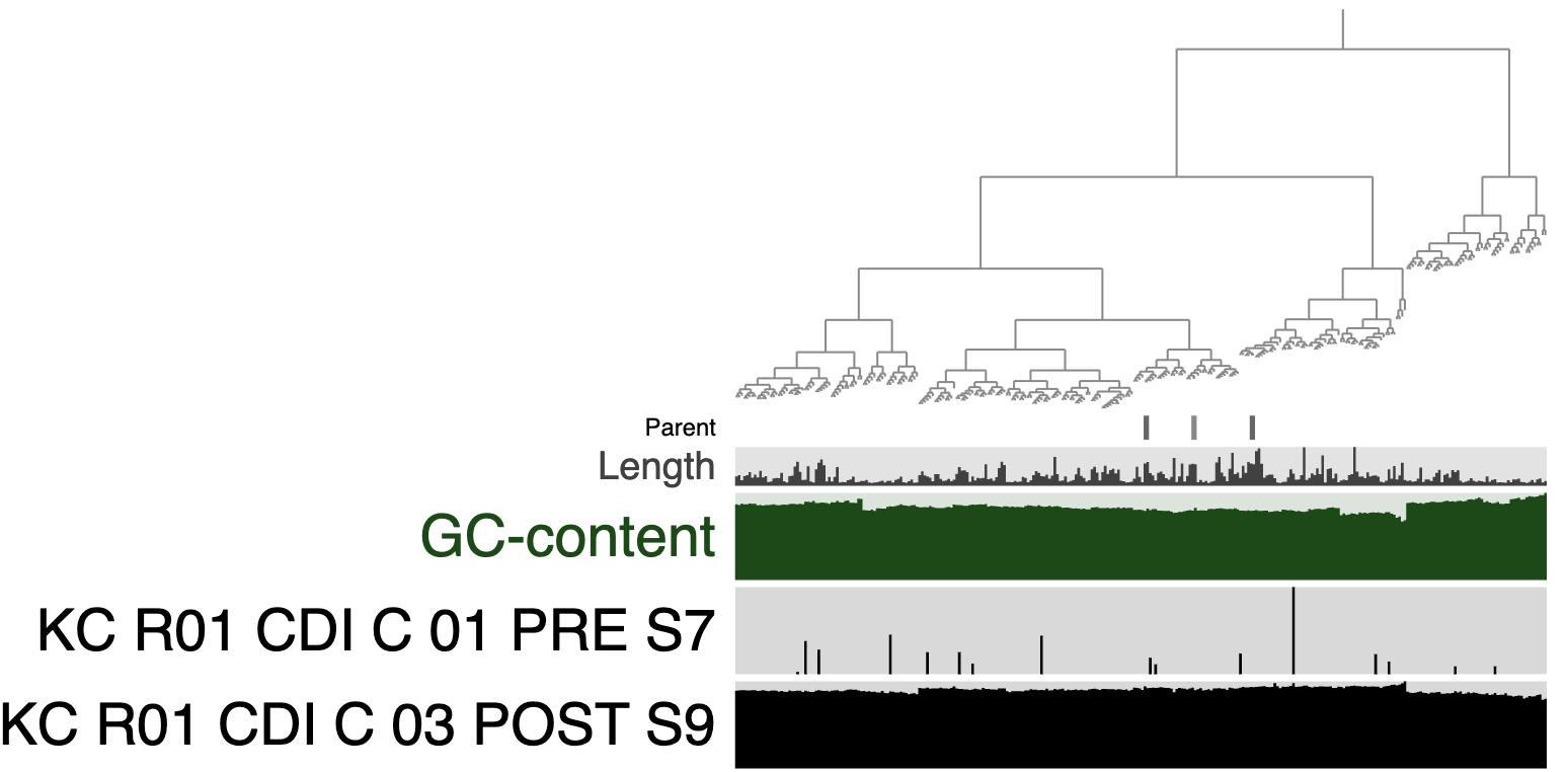
Does the MAG FMT_HIG_FITNESS_KC_MAG_00120 appear to colonize? What explanation is there for the mapping results from the pre-FMT metagenome?
At this point you have completed all of the computational steps to exploring the ecology of a MAG across two metagenomes. However, this analysis can be scaled up using our Snakemake workflows! We already ran the calculations for you, but here is what the read recruitment data from all 20 MAGs across these 2 metagenomes looks like:
anvi-interactive -d big_data/SUMMARY/bins_across_samples/mean_coverage.txt \
                 -p profile_mean_coverage.db \
                 --title "twenty_MAGs" \
                 --manual \
                 --state-autoload DFI

Which MAGs represent populations that colonized this recipient after FMT?
Part III: Investigating metabolism in MAGs (15 min)
In this section of the workshop, we’ll be estimating the metabolic capacity of the bacterial populations living in one FMT donor. As discussed in the lecture, we have 20 MAGs to compare - 10 that are considered ‘high-fitness’ colonizers and 10 that are considered ‘low-fitness’ non-colonizers. The datapack contains contigs databases for 19 of these MAGs, and a FASTA file for the last one, KC_MAG_00120, which you earlier converted into its own contigs database.
If you didn’t go through Part I, or if you didn’t download the KEGG database onto your computer by running anvi-setup-kegg-kofams, you can find a pre-annotated contigs database for KC_MAG_00120 in the backup_data/ folder of the datapack. In this case, we suggest copying it to your current directory by running cp backup_data/FMT_HIG_FITNESS_KC_MAG_00120.db . (you must include the final . in that command).
If you’re interested in this section of the workshop, a more comprehensive tutorial using a larger version of this dataset can be found here.
Annotate genes in the MAG with KEGG KOfams (~5 min)
In order to estimate metabolism in anvi’o v7, you need to annotate the genes in your genome with enzymes from the KEGG KOfam database. You can do this by running:
anvi-run-kegg-kofams -c FMT_HIG_FITNESS_KC_MAG_00120.db \
                 -T $THREADS
Reminder: skip the above command if you decided not to run anvi-setup-kegg-kofams, and use the pre-annotated, backup_data/ version of this database instead for the rest of the workshop.
That command will take about 5 minutes, given 4 threads. If you have more cores, you can increase the number of threads to make it go faster.
Once it is done running, you can inspect the database again - you should now see the annotations we added:
anvi-db-info FMT_HIG_FITNESS_KC_MAG_00120.db
Estimating metabolism (~3 min)
We have the enzyme annotations we need, so now we can use the following program to predict the metabolic capacity of our MAG:
anvi-estimate-metabolism -c FMT_HIG_FITNESS_KC_MAG_00120.db \
                 -O KC_MAG_00120
Take a look at the resulting file with
head KC_MAG_00120_modules.txt
You can also import this file into Excel if you prefer. We’ll discuss what the output means during the workshop (but you can also check the documentation here).
Our goal is to compare the metabolic capacities of all of these MAGs. The other databases have already been annotated properly, so they are ready for estimation. We can use the same input file we used before to run estimation on all of the MAGs:
anvi-estimate-metabolism -e external-genomes.txt \
                 -O FMT
Visualizing a heatmap of metabolic completeness across MAGs (~5 min)
If you’re the kind of person who likes looking at pictures rather than text and numbers, you might find it easier to convert the metabolism estimation output into a heatmap of module completeness scores. You can do this by first estimating metabolism with the --matrix-format flag to get a matrix file of just the completeness scores (no extra info), and then giving that file to anvi-interactive using the --manual-mode flag for visualizing ad hoc data files.
Here are the commands for this:
# 1) get the same metabolism estimation values, but formatted as a matrix
anvi-estimate-metabolism -e external-genomes.txt \
                 -O FMT \
                 --matrix-format

# 2) the output file we want is FMT-completeness-MATRIX.txt, check it out:
head FMT-completeness-MATRIX.txt

# 3) use the matrix to make a dendrogram that organizes modules by their patterns of completeness across MAGs
anvi-matrix-to-newick FMT-completeness-MATRIX.txt

# 4) visualize (you must provide a name for a new profile database that can be used to store visualization information if necessary)
anvi-interactive -A FMT-completeness-MATRIX.txt \
                 -t FMT-completeness-MATRIX.txt.newick \
                 -p FMT-completeness-MATRIX_profile.db \
                 --manual-mode \
                 --title "Heatmap of module completeness scores across MAGs"
In the interactive interface in your browser, there are a lot of settings you can change to get this looking like a heatmap. For example, I always change the ‘Drawing type’ to be ‘Phylogram’ so that it is a rectangle instead of a circle. I also always change the bar graphs into intensities (with a min of 0 and a max of 1). We will go over how to do this in the workshop.
In the datapack, I’ve provided a profile database that contains some saved settings (a ‘state’, in anvi’o lingo) to make this heatmap look super pretty. Here is how you can look at it:
anvi-interactive -A FMT-completeness-MATRIX.txt \
                 -t FMT-completeness-MATRIX.txt.newick \
                 -p backup_data/FMT-completeness-MATRIX_profile.db \
                 --manual-mode \
                 --title "Heatmap of module completeness scores across MAGs"

To make it look this nice, here are some of the additional things I added:
- a dendrogram organizing the MAGs according to the distribution of module completeness scores (so MAGs that have similar metabolic capabilities will be closer together)
- colors to indicate which MAGs are high-fitness and which MAGs are low-fitness
- the names and categories of modules so that we can see what pathway each one represents (instead of just the module identifier)
If you hover your mouse over the various boxes in the heatmap and look at the ‘Mouse’ tab, you will see that there is even more information available for each MAG and pathway - they just aren’t visible. You can make them visible by increasing the ‘height’ settings for those layers (so that they are non-zero).
Anyway, if you look at the prettified heatmap, you should notice a block of metabolic modules that are highly complete in the high-fitness MAGs, but largely missing from the low-fitness MAGs. What are these pathways?
In the next section, we’re going to learn how to mathematically find these pathways that are over-represented in the high-fitness group, by computing an enrichment score.
Computing enrichment of metabolic pathways in groups of genomes (~2 min)
You might recall that our MAGs belong to two different groups - 10 are ‘high-fitness’ and 10 are ‘low-fitness’. To compare the metabolic capacities of the two groups, we can do statistical tests to figure out which metabolic pathways are over-represented in one group or another. The program that does this enrichment analysis is called anvi-compute-metabolic-enrichment.
In order to run the enrichment analysis, we need to specify which group each MAG belongs to. Luckily, this information is already in the metadata file:
head MAG_metadata.txt # see the columns 'name' and 'group'
The metadata file can serve as our ‘group’ file. We give that file, along with the metabolism estimation output, to this program:
anvi-compute-metabolic-enrichment -M FMT_modules.txt \
                 -G MAG_metadata.txt \
                 -o metabolic_enrichment.txt
Please note that the name of each MAG must be the same in both files. If you named your KC_MAG_00120 database as we suggested, you should not have any problem. But if you named it differently, you should change the corresponding name in the metadata file to match its name in the metabolism output file.
Take a look at metabolic_enrichment.txt. What do you notice? (Hint: check the associated_groups column)
| KEGG_MODULE | enrichment_score | unadjusted_p_value | adjusted_q_value | associated_groups | accession | sample_ids | p_FMT_HIGH_FITNESS | N_FMT_HIGH_FITNESS | p_FMT_LOW_FITNESS | N_FMT_LOW_FITNESS |
|---|---|---|---|---|---|---|---|---|---|---|
| Adenine ribonucleotide biosynthesis, IMP => ADP,ATP | 19.99999999999999 | 7.744216431044125e-6 | 2.1088636680069928e-5 | FMT_HIGH_FITNESS | M00049 | KC_MAG_00022,KC_MAG_00051,KC_MAG_00055,KC_MAG_00116,KC_MAG_00120,KC_MAG_00145,KC_MAG_00147,KC_MAG_00151,KC_MAG_00162,KC_MAG_00178 | 1 | 10 | 0 | 10 |
| Coenzyme A biosynthesis, pantothenate => CoA | 19.99999999999999 | 7.744216431044125e-6 | 2.1088636680069928e-5 | FMT_HIGH_FITNESS | M00120 | KC_MAG_00022,KC_MAG_00051,KC_MAG_00055,KC_MAG_00116,KC_MAG_00120,KC_MAG_00145,KC_MAG_00147,KC_MAG_00151,KC_MAG_00162,KC_MAG_00178 | 1 | 10 | 0 | 10 |
| Guanine ribonucleotide biosynthesis IMP => GDP,GTP | 19.99999999999999 | 7.744216431044125e-6 | 2.1088636680069928e-5 | FMT_HIGH_FITNESS | M00050 | KC_MAG_00022,KC_MAG_00051,KC_MAG_00055,KC_MAG_00116,KC_MAG_00120,KC_MAG_00145,KC_MAG_00147,KC_MAG_00151,KC_MAG_00162,KC_MAG_00178 | 1 | 10 | 0 | 10 |
| Pentose phosphate pathway, non-oxidative phase, fructose 6P => ribose 5P | 19.99999999999999 | 7.744216431044125e-6 | 2.1088636680069928e-5 | FMT_HIGH_FITNESS | M00007 | KC_MAG_00022,KC_MAG_00051,KC_MAG_00055,KC_MAG_00116,KC_MAG_00120,KC_MAG_00145,KC_MAG_00147,KC_MAG_00151,KC_MAG_00162,KC_MAG_00178 | 1 | 10 | 0 | 10 |
| C5 isoprenoid biosynthesis, non-mevalonate pathway | 16.363709270757376 | 5.227664682736589e-5 | 7.11784866558805e-5 | FMT_HIGH_FITNESS | M00096 | KC_MAG_00022,KC_MAG_00051,KC_MAG_00055,KC_MAG_00116,KC_MAG_00145,KC_MAG_00147,KC_MAG_00151,KC_MAG_00162,KC_MAG_00178 | 0.9 | 10 | 0 | 10 |
| F-type ATPase, prokaryotes and chloroplasts | 16.363709270757376 | 5.227664682736589e-5 | 7.11784866558805e-5 | FMT_HIGH_FITNESS | M00157 | KC_MAG_00022,KC_MAG_00051,KC_MAG_00055,KC_MAG_00116,KC_MAG_00120,KC_MAG_00145,KC_MAG_00147,KC_MAG_00151,KC_MAG_00178 | 0.9 | 10 | 0 | 10 |
| Inosine monophosphate biosynthesis, PRPP + glutamine => IMP | 16.363709270757376 | 5.227664682736589e-5 | 7.11784866558805e-5 | FMT_HIGH_FITNESS | M00048 | KC_MAG_00022,KC_MAG_00051,KC_MAG_00055,KC_MAG_00116,KC_MAG_00120,KC_MAG_00147,KC_MAG_00151,KC_MAG_00162,KC_MAG_00178 | 0.9 | 10 | 0 | 10 |
| Uridine monophosphate biosynthesis, glutamine (+ PRPP) => UMP | 16.363709270757376 | 5.227664682736589e-5 | 7.11784866558805e-5 | FMT_HIGH_FITNESS | M00051 | KC_MAG_00022,KC_MAG_00051,KC_MAG_00055,KC_MAG_00116,KC_MAG_00120,KC_MAG_00145,KC_MAG_00147,KC_MAG_00151,KC_MAG_00178 | 0.9 | 10 | 0 | 10 |
| Histidine biosynthesis, PRPP => histidine | 13.333348987572858 | 2.6072745627699713e-4 | 1.7749977182659536e-4 | FMT_HIGH_FITNESS | M00026 | KC_MAG_00022,KC_MAG_00051,KC_MAG_00116,KC_MAG_00120,KC_MAG_00147,KC_MAG_00151,KC_MAG_00162,KC_MAG_00178 | 0.8 | 10 | 0 | 10 |
Takeaways
Today we used genomics and metagenomics to explore the colonization of bacteria after FMT and investigated fitness-determining genomic characteristics that may have contributed to their success or failure.
We hope anvi’o helped you along the way and you can find some new ways to analyze your own data! If you have any questions about anvi’o and want to join the community please check out our slack channel!