An Akkermansia story with MinION long-reads

Table of Contents
Summary
The purpose of this worklfow is to walk you through an application of metagenomics long-read sequencing. Throughout this exercise you will learn about,
- High molecular weight DNA extraction, for metagenomics applications,
- Assembly of long-read metagenome and the recovery of circular genomes,
- How to correct long-reads contigs, with or without short-reads,
- Use anvi’o pangenomics workflow to assess long-read correction,
- Compare long-read assembled genomes with reference genomes.
If you have any questions about this exercise, or have ideas to make it better, please feel free to get in touch with the anvi’o community through our Discord server:

To reproduce this exercise with your own dataset, you should first follow the instructions here that will install anvi’o.
Once you have anvi’o successfully installed, you will need to install additional software (not needed to complete this tutorial): metaFlye, minimap2, Pilon and proovframe.
Downloading the data pack
First, open your terminal, go to a work directory, and download the data pack we have stored online for you:
curl -L https://cloud.uol.de/public.php/dav/files/aWDr8ECXA5a7CdJ \
     -o LONG_READ_METAGENOMICS.tar.gz
Then unpack it, and go into the data pack directory:
tar -zxvf LONG_READ_METAGENOMICS.tar.gz

cd LONG_READ_METAGENOMICS
At this point, if you type ls in your terminal, this is what you should be seeing:
ANVIO_DATABASES FILES GENOMES
These are the directories that include databases for anvio pangeomes (i.e., anvi’o artifacts called pan-db and genomes-storage-db), config files, as well as FASTA files for genomes.
Let’s first create an environmental variable to be able to access the working directory path rapidly:
export WD=`pwd`
Watson et al. 2021: A Fecal Microbiota Transplantation
This tutorial is based on a recent study on fecal microbiota transplantation (FMT), in which patients with Clostridium difficile infection get a microbiota transfer from a healthy donor.
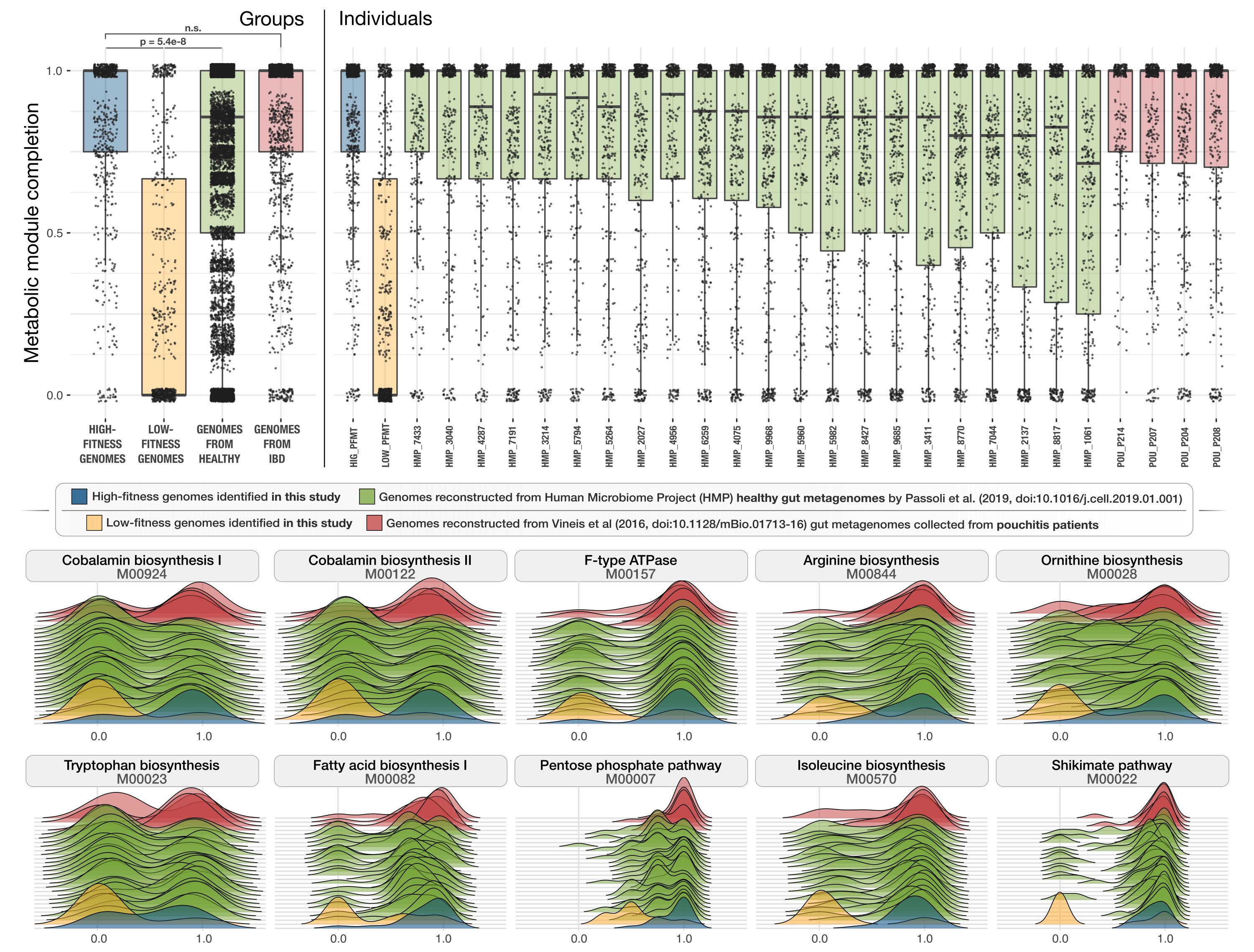
- Includes an observation that links the presence of superior metabolic competence in bacterial populations to their expansion in IBD.
- Here is a Twitter thread that explains key points of the study.
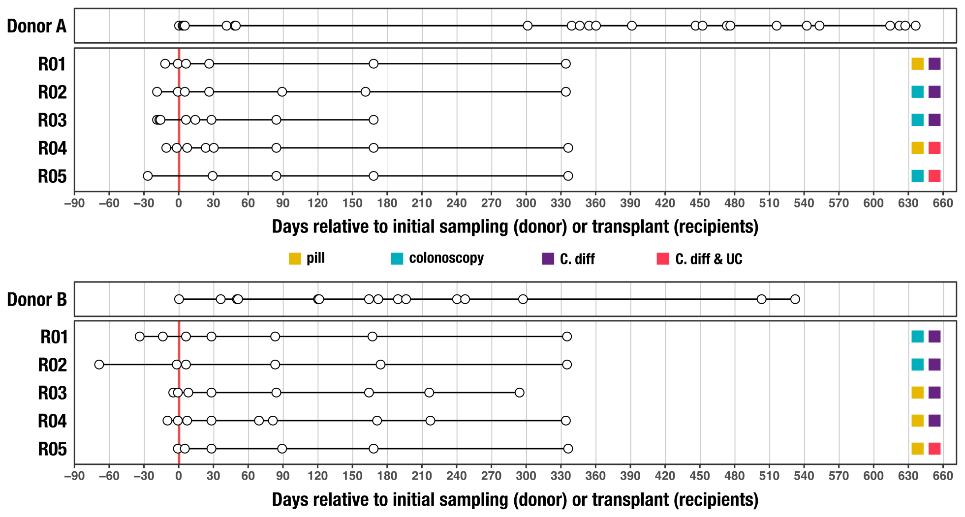
An objective of this study was to better understand determinants of microbial colonization in the human gut. FMT is a powerful framework to study such questions since it enables precise tracking of donor microbial populations and colonization events in recipient guts. With the time-series data we have generated for our study, we could also interrogate long-term outcomes of such colonization events (or lack thereof). In brief, the data consists of shotgun metagenomic sequencing of poop samples collected from the donors and the FMT recipients before and after FMT:
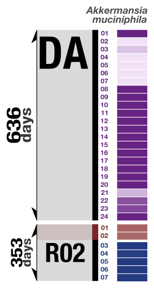
We performed a co-assembly of each donor metagenome, and used a combination of automatic and manual binning strategies to obtain 128 high-quality metagenome-assembled genomes (MAGs) from Donor A, one of the donors that we will focus on in this tutorial. Here is a heatmap representing the detection of these 128 MAGs in the donor and recipient metagenomes:

Here we are particularly interested in a population from the phylum Verrucomicrobia that resolves to the species Akkermansia muciniphila. We detected the MAG for this population both in many samples from the donor as well as in many recipients post-FMT. But for the second recipient, we noticed that the donor MAG recruited reads also from pre-FMT metagenomes, suggesting the presence of a similar population in this recipient prior to FMT:
Given this interesting dynamic, a question that has a lot of value for a study that investigates microbial colonization begs an answer: did the donor Akkermansia muciniphila population replace the recipient population, or did the recipient population that existed pre-FMT manage to persist and fend off the donor population? We could answer this question very rapidly using single-nucleotide variants. This would have been quite straightforward given the program anvi-gen-variability-profile which gives access to a comprehensive microbial population genetics framework in anvi’o.
But if we wish to investigate genomic differences between these closely related pre-FMT and post-FMT populations that may explain some of the determinants of their success over one another, we would need more than SNVs. Preferably, complete genomes! So to achieve that, we decided to use long-read sequencing (MinION) to characterize metagenomes that may help us in the quest of recovering complete Akkermansia muciniphila genomes.
A few words on high molecular weight DNA extraction strategies
Oxford Nanopore Technology offers new opportunities with the sequencing of very long DNA fragments. In fact there is no theoretical limit for the reads length, but the real world is cruel and read lengths are rarely infinite. The major reason for that read length limitation lies in the DNA extraction, for which we can observe a great revival of interest. For years, DNA extraction protocols and commercial kits have been optimized to provided the best DNA yields and cope with sample specific limitations (matrix/inhibitors) without any considerations for the high molecular weight DNA fraction. Especially since most short-reads sequencing strategies use DNA fragmentation and size-selection to narrow the insert-size and facilitate downstream analysis.
Now we are interested in DNA extraction methods to recover the longest DNA fragments, and one of the best methods is a good old phenol/chloroform extraction. Variations of this protocol are regularly used for isolate genome sequencing, and it generates the required read lengths to reconstruct complete and circular genomes.
It was only a matter of time before people interested in more complex samples started to use long-read sequencing for metagenomics analysis. And naturally, they used the same DNA extraction methods as used for isolate genome sequencing. And it makes sense given the extra-long DNA fragments produced by this method. But should we only focus on maximum length possible when it comes to metagenomics?
We conducted a study to compare different high molecular weight DNA extraction strategies, using relatively low biomass and host-contaminated sample: tongue scraping.
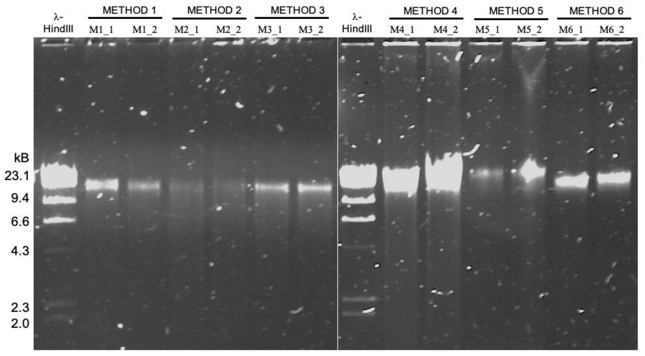
- It turns out the protocol that works best for sequencing DNA from microbial isolates may not be the most effetive method for long-read sequencing of metagenomes ¯\_(ツ)_/¯
We compared the read length distribution and their downstream consequences from a metagenomics point of view (microbial diversity recovered, amount of host contamination, assembly metrics).
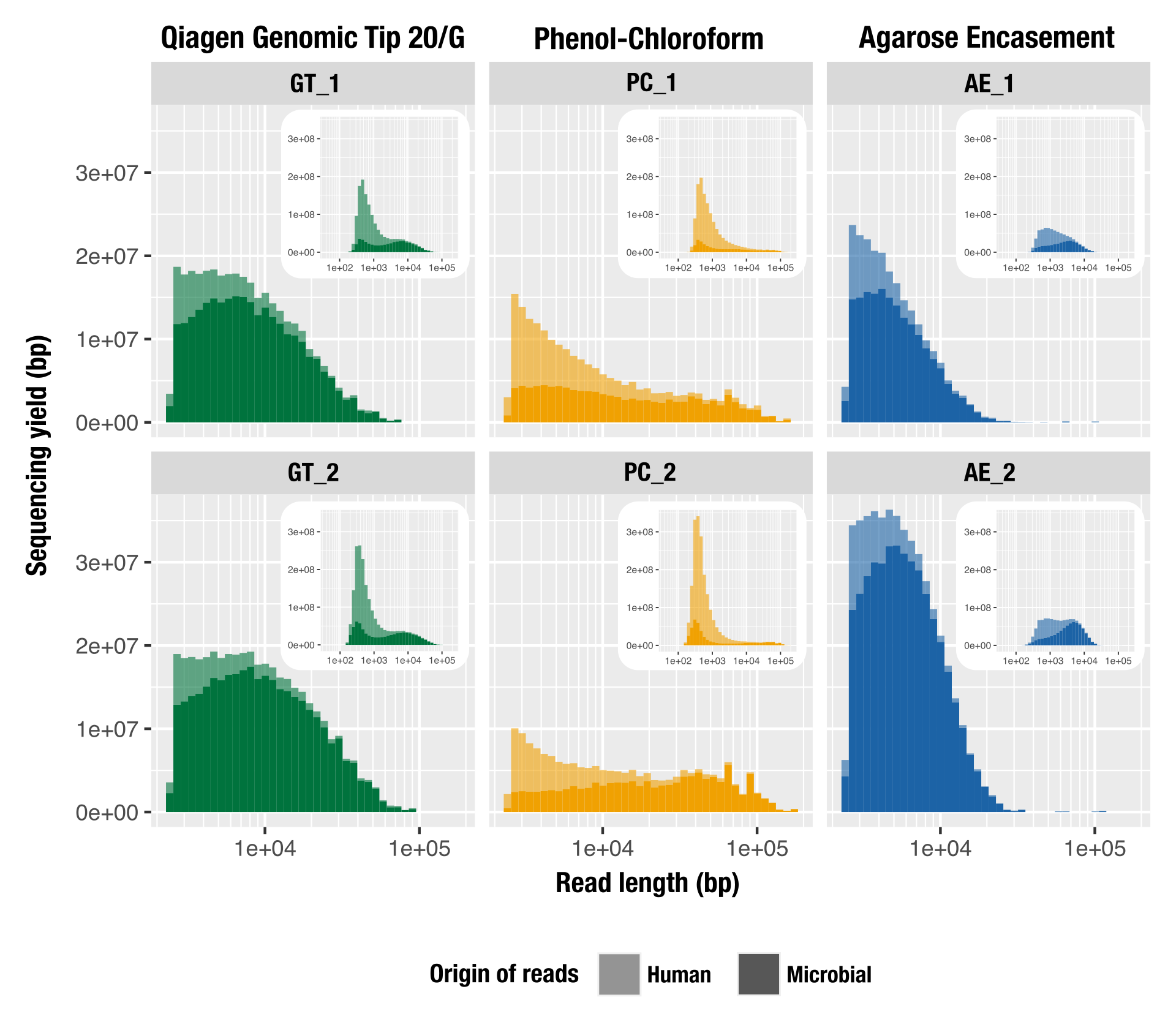
Phenol-chloroform extraction is frequently endorsed for its ability to produce extremely long DNA fragments for long-read sequencing, which was also the case in our study as PC yielded the longest fragments we sequenced. But we also found that modified versions of commercially available column-based and agarose-based extraction methods outperform phenol-chloroform long-read sequencing of metagenomes. In this pool of extraction methods, the Qiagen Genomic Tip 20/G extraction kit augmented with additional enzymatic cell lysis was the best approach to generate high-quality input DNA from complex metagenomes for long-read sequencing.
We applied shotgun metagenomic long-read sequencing to three samples from Recipient 2: before FMT (-1), right after FMT (+5 days), and almost a year post-FMT (+334 days). The table below shows some brief statistics for each MinION run:
| Sample | W0 | W1 | W48 |
|---|---|---|---|
| DNA concentration (ng/µl) | 30.2 | 17.1 | 52.9 |
| Sequencing yield (Mbp) | 10,499 | 4,282 | 10,596 |
| Number of reads | 6,292,659 | 3,964,054 | 6,263,555 |
| N50 (bp) | 3,156 | 1,465 | 4,177 |
Metagenomics Long-Read Assembly
In this part of the tutorial, we will go through the commands used to generate the long-read assembly. The raw reads are not provided here but these commands could be useful if you want to apply the same analysis with your own data
Long-read assembly is quite different from short-read assembly simply due to the high error rate inherent to the Nanopore sequencing. As a result, a new field of long-read assemblers emerged in the last decade, like miniasm, Canu, Flye, wtdbg2, Falcon or OPERA-MS. Unfortunately for us, they were designed for whole genome assembly and not really for metagenomics. The main difference is the ability for an assembler to deal with the multiple levels of coverage in metagenomes compared to samples with only one microbial population.
But as was the case for short-read assemblers, there are now a few options for metagenomic long-reads! For instance, Canu and wtdbg2 are able to deal with metagenomes with a few changes in the default parameters, but there is one assembler that was designed specifically for metagenomes: metaFlye (actually Flye for metagenomes). We are using the latter with our dataset, but feel free to try different assemblers for your own dataset.
metaFlye assembly
Using Flye is quite straightforward. It is one command only and just requires your raw long-reads and the --meta flag.
While it looks simple, there are multiple steps that are run in the background.
Briefly, it counts and filters out erroneous k-mers and extends contigs using the “good k-mer”. It then aligns the long reads with minimap2 to resolve repeats, and finally, runs a polishing step to correct sequencing errors.
You should not run the commands displayed in these blue boxes. These commands are only here to illustrate the softwares used to generate the data provided for this tutorial.
flye --nano-raw /path/to/your/long-reads/sample.fastq \
     --out-dir 01_ASSEMBLY_META \
     --meta \
     -t 8
Among the output files, you can find the fasta file with the contigs, the assembly graph file, and also a summary table for each contig. That summary file contains the contig ID, length, coverage, circularity, presence of repetitions and a few other pieces of information.
We generated contigs databases with anvi’o workflow for each assembly and used anvi-estimate-scg-taxonomy to get the taxonomy for each contig. Here are the summary tables for each of the three assemblies (5 largest contigs):
| W0 | length | cov. | circ. | taxonomy |
|---|---|---|---|---|
| contig_3 | 5311782 | 723 | + | Enterobacteriaceae |
| contig_5 | 5034533 | 215 | + | Enterobacteriaceae |
| contig_49 | 2956370 | 989 | + | Akkermansia muciniphila |
| contig_84 | 1985221 | 55 | + | Pediococcus acidilactici |
| contig_75 | 1907875 | 476 | + | Dialister invisus |
| W1 | length | cov. | circ. | taxonomy |
|---|---|---|---|---|
| contig_117 | 3831826 | 32 | - | Tyzzerella nexilis |
| contig_473 | 3067601 | 56 | + | Akkermansia muciniphila |
| contig_18 | 2930711 | 92 | - | Faecalicatena torques |
| contig_97 | 2894730 | 54 | - | Blautia sp000432195 |
| scaffold_824 | 2847284 | 24 | - | Absiella |
| W48 | length | cov. | circ. | taxonomy |
|---|---|---|---|---|
| contig_40 | 3541224 | 1120 | + | Agathobacter |
| contig_177 | 3440959 | 18 | - | Eggerthella lenta |
| contig_18 | 3249686 | 25 | - | CAG-41 sp900066215 |
| contig_332 | 3067113 | 47 | + | Akkermansia muciniphila |
| contig_13 | 2921266 | 60 | + | Faecalicatena torques |
Akkermansia muciniphila genome correction
We have identified three circular genomes of Akkermansia muciniphila from three different samples. We will use the anvi’o pangenomics workflow to compare these genomes before and after two types of long-read assembly correction.
Compare the raw genomes
Before any polishing/correction, it is interesting to compare the raw genomes. We will learn about the impact of high error rate (especially indels) in a comparative genomics analysis. We are going to use the pangenomics snakemake workflow in anvi’o, so let’s start by activating the anvi’o environment and create a directory for the pangenome of the raw Akkermansia muciniphila genomes:
conda activate anvio-7.1

mkdir -p PAN_RAW && cd PAN_RAW
We can use the help menu for anvi-run-workflow
anvi-run-workflow -h
Let’s generate a config file:
anvi-run-workflow -w pangenomics --get-default-config config_raw.json
We should modify the config_raw.json to include appropriate thread count for each step of the workflow and also remove unused command (optional, but it can make is easier to read and understand the config file).
You can copy an existing config file:
cp $WD/FILES/config_raw.json .
We also need a fasta_raw.txt, which should be a two columns file with the name of our genomes and their path.
cp $WD/FILES/fasta_raw.txt .
cat fasta_raw.txt
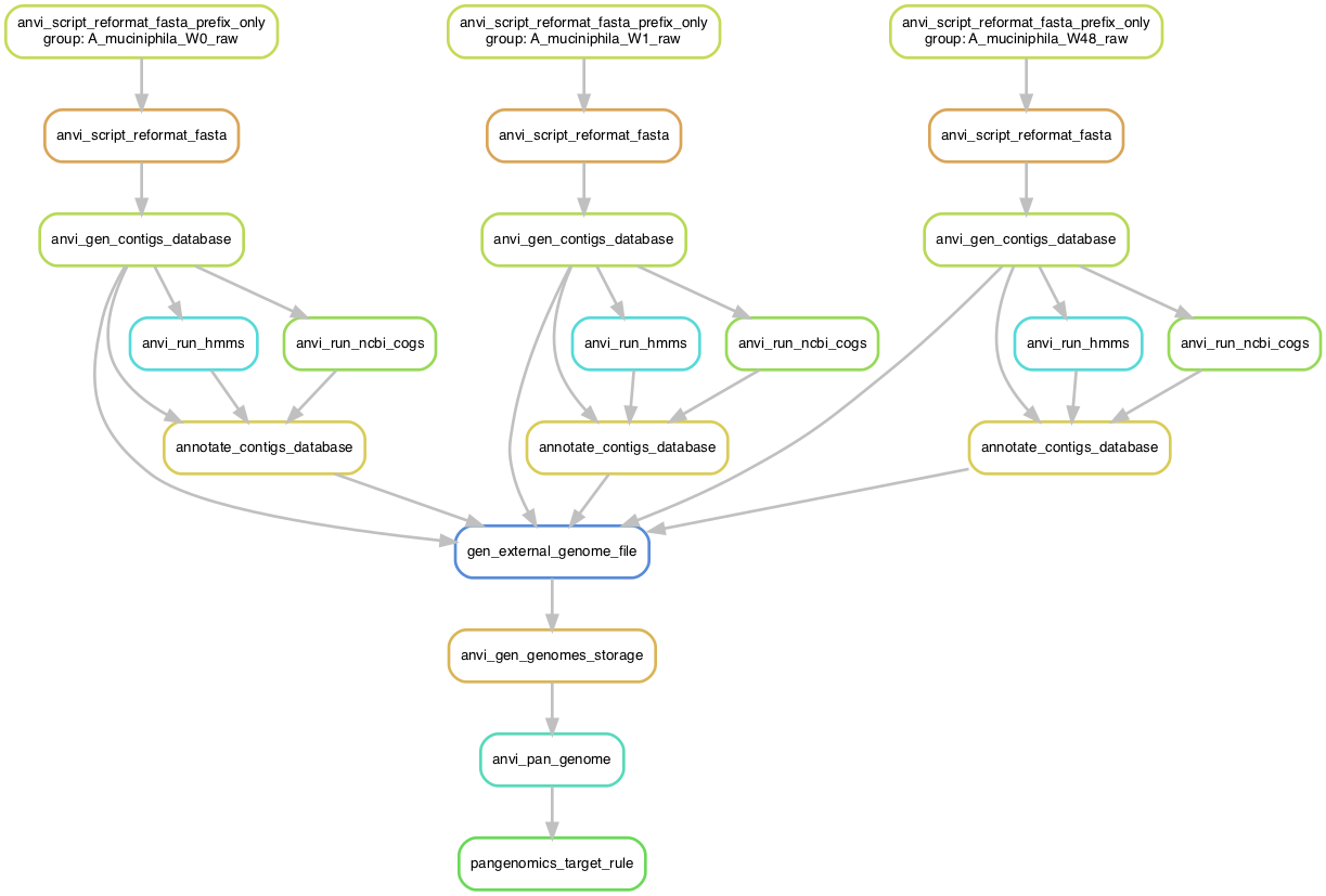
We can generate a workflow graph to see all of the steps that will be run on the machine:
anvi-run-workflow -w pangenomics -c config_raw.json --save-workflow-graph

open workflow.png
Let’s run the workflow now:
anvi-run-workflow -w pangenomics -c config_raw.json
Once the workflow is complete, we can use anvi’o to visualize the pangenome:
anvi-display-pan -g 03_PAN/A_muciniphila_Raw-GENOMES.db -p 03_PAN/A_muciniphila_Raw-PAN.db
Show/hide Akkermansia muciniphila raw pangenome

Homework: make your pangenome look like this one. Here are the color codes used for each layer:
| Layer | Hex color |
|---|---|
| W0 | 2e4552 |
| W1 | 4b9b8f |
| W48 | 4b9b8f |
| Geometric homogeneity | d87559 |
| SCGs bin | e8a56b |
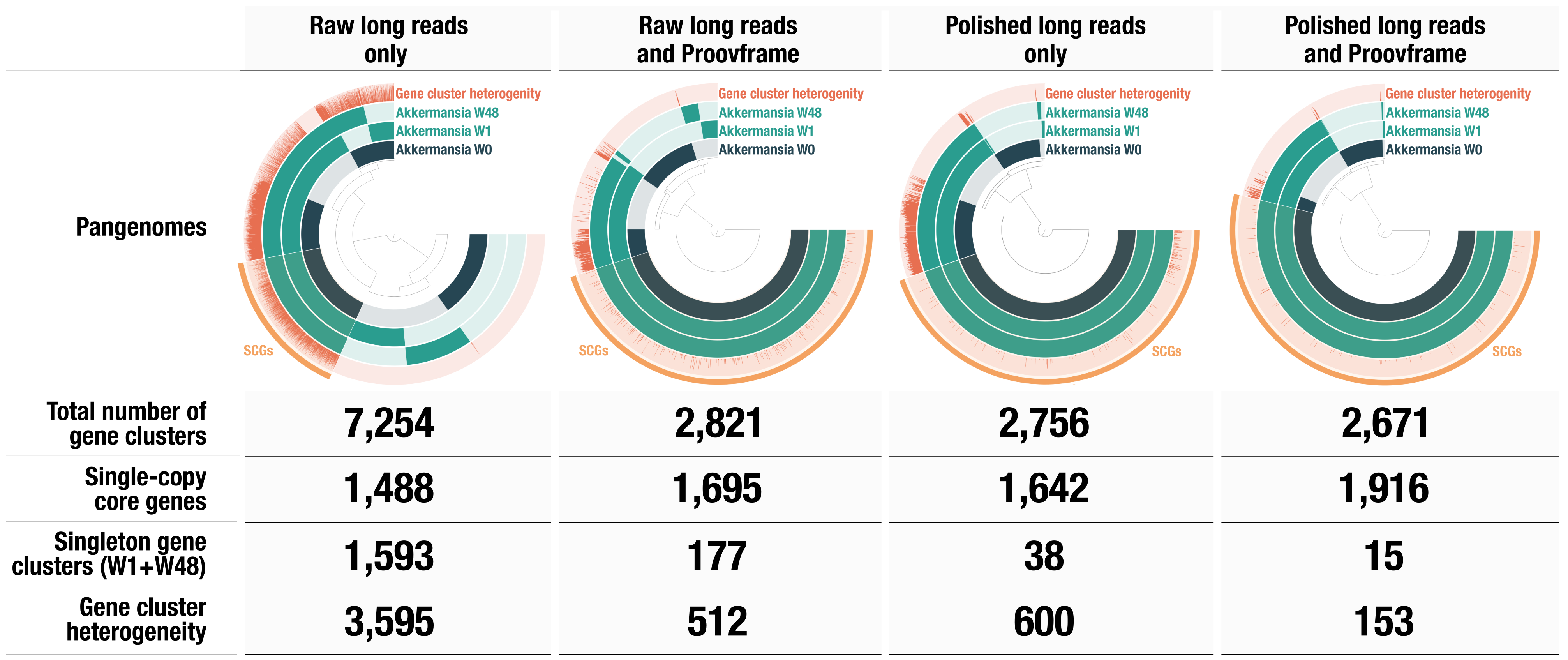
There are 7,254 total gene clusters (GCs), of which 1,488 are single-copy core genes. We can see that there is a large fraction of gene clusters unique to each genome, suggesting that there are some differences between each of them. We can also compute the average nucleotide identity and add it as an additional table to the pangenome database and visualize it in the interactive interface:
anvi-compute-genome-similarity -p 03_PAN/A_muciniphila_Raw-PAN.db -e external-genomes.txt -o 04_ANI
The percent identity matrix should look like this:
cat 04_ANI/ANIb_percentage_identity.txt
| key | A_muciniphila_W0_raw | A_muciniphila_W1_raw | A_muciniphila_W48_raw |
|---|---|---|---|
| A_muciniphila_W0_raw | 1.0 | 0.8786730791912385 | 0.8789288242730721 |
| A_muciniphila_W1_raw | 0.8788478088480801 | 1.0 | 0.9943445872170439 |
| A_muciniphila_W48_raw | 0.8790883856127144 | 0.994327842876165 | 1.0 |
And the alignment coverage:
cat 04_ANI/ANIb_alignment_coverage.txt
| key | A_muciniphila_W0_raw | A_muciniphila_W1_raw | A_muciniphila_W48_raw |
|---|---|---|---|
| A_muciniphila_W0_raw | 1.0 | 0.7976643654211076 | 0.7972337697920084 |
| A_muciniphila_W1_raw | 0.7740364538934497 | 1.0 | 0.9957432534413699 |
| A_muciniphila_W48_raw | 0.7723099866225992 | 0.996145887027964 | 1.0 |
And run the interactive interface again:
anvi-display-pan -g 03_PAN/A_muciniphila_Raw-GENOMES.db \
                 -p 03_PAN/A_muciniphila_Raw-PAN.db
Show/hide Akkermansia muciniphila raw pangenome with ANI
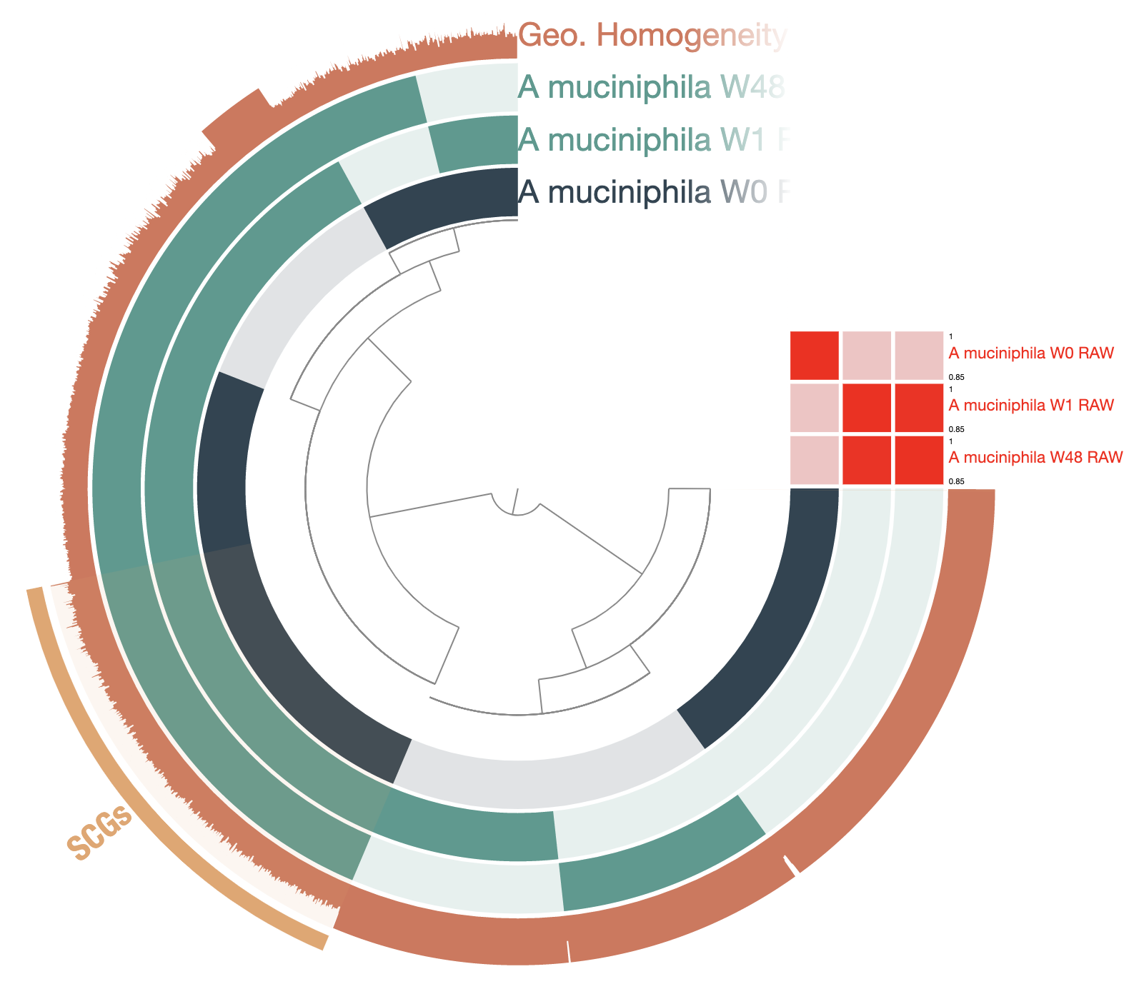
So, W0 is actually very different from W1 and W48. But the later genomes are practically identical according to the ANI. Most of the singleton GCs were fragmented genes, which results from the low quality of the MinION reads and contigs. The most common errors are indels, which disrupt open reading frames. One solution is to polish the genomes, using high quality short-reads, for example.
Pilon: use short-reads to polish genomes
Using Pilon
We used the short-read metagenomes from Watson et al. to polish the assemblies. These steps are quite resource intensive, so we directly provided you with the polished genomes. Nevertheless, you can find all the commands used to generate the polished version of the three Akkermansia muciniphila genomes here.
We used Pilon to correct the metagenomics contigs. It requires you to map the short-reads to the long-reads contigs, for which you can use any of your favorite mapping software. In this case, I used minimap2. Then, we need to sort and index the bam files and finally, run pilon. In this example, I’ve used a for loop to polish the three genomes. Of course, you should replace the path to each genome and the associated short-reads for the command to run. This is just an example:
# map the short-reads to the assembly
minimap2 -t 4 -ax map-ont path/to/your/assembly.fasta \
         path/to/your/sort-read-R1.fastq \
         path/to/your/sort-read-R2.fastq \
         > short_read_mapping.sam

# convert and sort the sam file
samtools sort short_read_mapping.sam \
         -@ 4 -o short_read_mapping.bam

# index the bam file
samtools index short_read_mapping.bam

# run pilon
java -Xmx16G -jar path/to/pilon/pilon-1.24-0/pilon.jar \
             --genome path/to/your/assembly.fasta \
             --bam short_read_mapping.bam \
             --outdir pilon \
             --output assembly_pilon
Let’s do another pangenome with the polished genomes now. Let’s first make sure we are working in the right directory:
cd $WD
We are going to skip some steps here and use pan & genomes databases that were already generated. But the concept is the same as for the first pangenome, we are just using the polished genomes instead. If you want to make the pan & genomes databases yourself, the genomes are available here: GENOMES/SR_POLISHED.
Anvi’o interactive interface:
anvi-display-pan -g ANVIO_DATABASES/02_SR_POLISHED/03_PAN/A_muciniphila-GENOMES.db \
                 -p ANVIO_DATABASES/02_SR_POLISHED/03_PAN/A_muciniphila-PAN.db
Show/hide Akkermansia muciniphila pangenome polished with Pilon
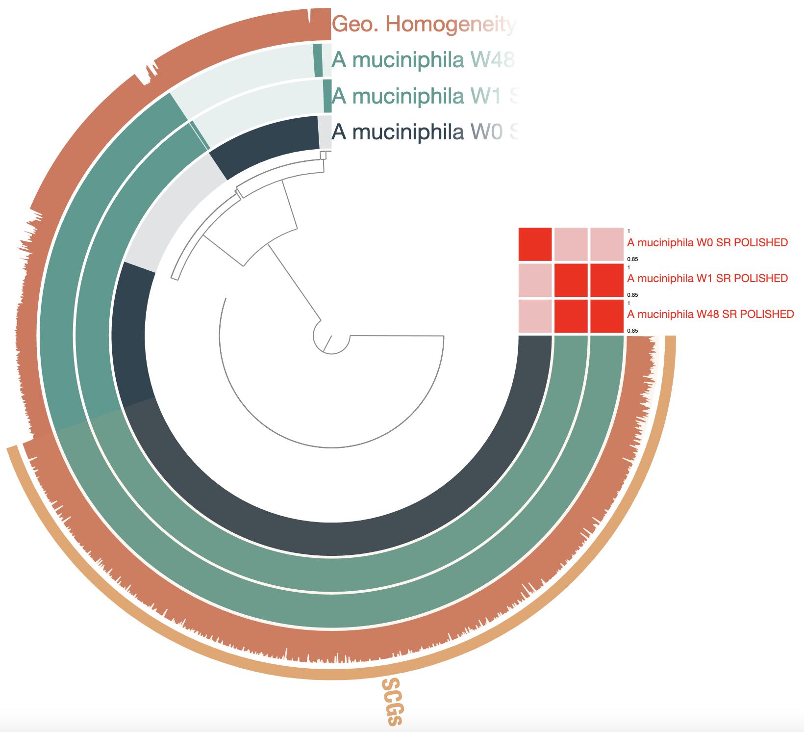
See anything different from the previous pangenome? The total number of GCs went from 7,254 to 2,756! The core is proportionally larger, which is more consistent with what we should expect from a species-level pangenome. The geometric homogeneity is also a lot higher, indicating better alignments. The polishing step dramatically improved the quality of these genomes from the point of view of the gene calling, therefore improving our ability to compare them based on their gene content.
The only issue here is that you need to have the associated short-reads to be able to polish your long-read assemblies. If you don’t have them, there is still a solution for you: proovframe. A tool to correct frameshift errors using a protein reference database.
Proovframe: correct frameshift errors
Using proovframe
Proovframe detects and corrects frameshifts in coding sequences.
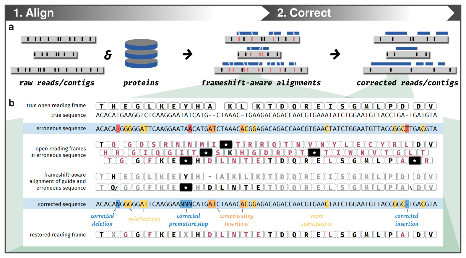
It can be used as an additional polishing step on top of classic consensus-polishing approaches for assemblies. It can be used on raw reads directly, which means it can be used on data lacking sequencing depth for consensus polishing - a common problem for a lot of rare things from environmental metagenomic samples, for example.
Like for the Pilon short-read polishing, this step can take some time and the database is quite large (uniref90), so we won’t run the commands. But for reproducibility, here are the steps we performed to correct the Akkermansia muciniphila genomes:
# first, proovframe maps proteins to contigs
# map proteins to reads
proovframe map -a /path/to/your/uniref/database/uniref90.fasta \
               -o proovframe/raw-seqs.tsv \
               -t 8 \
               path/to/your/assembly.fasta

# fix frameshifts in the contigs
proovframe fix -o proovframe/assembly_proovframe.fasta \
               path/to/your/assembly.fasta \
               proovframe/raw-seqs.tsv
The genomes corrected with proovframe can be found here: GENOMES/RAW_PF/
If you want to get your hands dirty, feel free to run the pangenomics workflow yourself with the availables genomes. But for now, we can stick to the existing anvi’o databases.
Let’s have a look at the new pangenome:
anvi-display-pan -g ANVIO_DATABASES/03_RAW_PF/03_PAN/A_muciniphila-GENOMES.db \
                 -p ANVIO_DATABASES/03_RAW_PF/03_PAN/A_muciniphila-PAN.db
Show/hide Akkermansia muciniphila pangenome corrected with proovframe
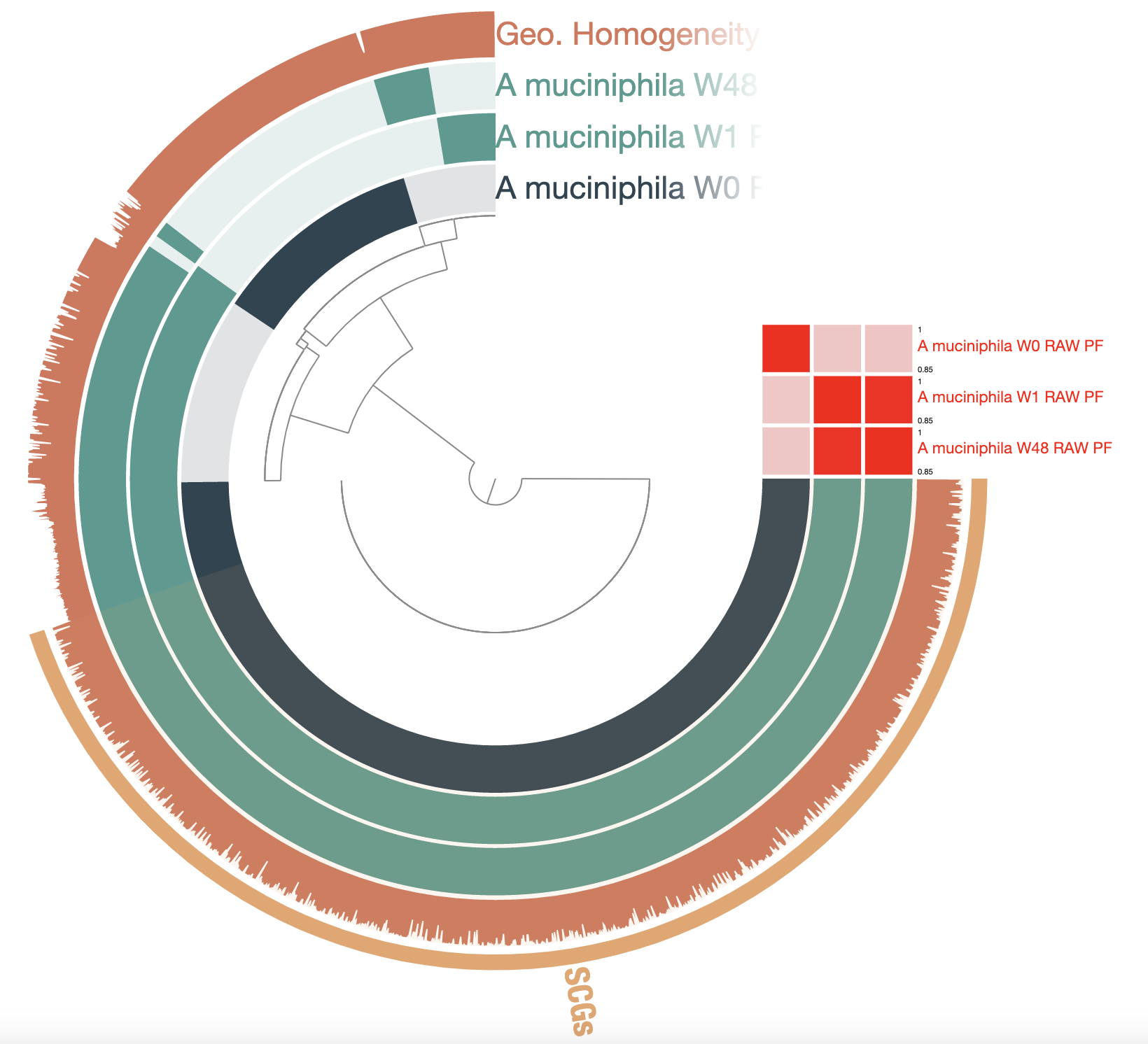
Not bad! Not far from the short-read polishing. We can observe the same reduction of total number of GCs and the increase of single copy core genes.
Combine Pilon and Proovframe
Because why not?
Let’s take the best of both worlds and see if we can improve a little bit further the quality of these genomes, especially W1 and W48, which are supposed to be virtually identical given their very high ANI.
Genomes that were corrected by both Pilon and proovframe can be found here: GENOMES/SR_POLISHED_PF/.
But once again, we will directly use the available pan and genomes databases:
anvi-display-pan -g ANVIO_DATABASES/04_SR_POLISHED_PF/03_PAN/A_muciniphila-GENOMES.db \
                 -p ANVIO_DATABASES/04_SR_POLISHED_PF/03_PAN/A_muciniphila-PAN.db
Show/hide Akkermansia muciniphila pangenome corrected with proovframe
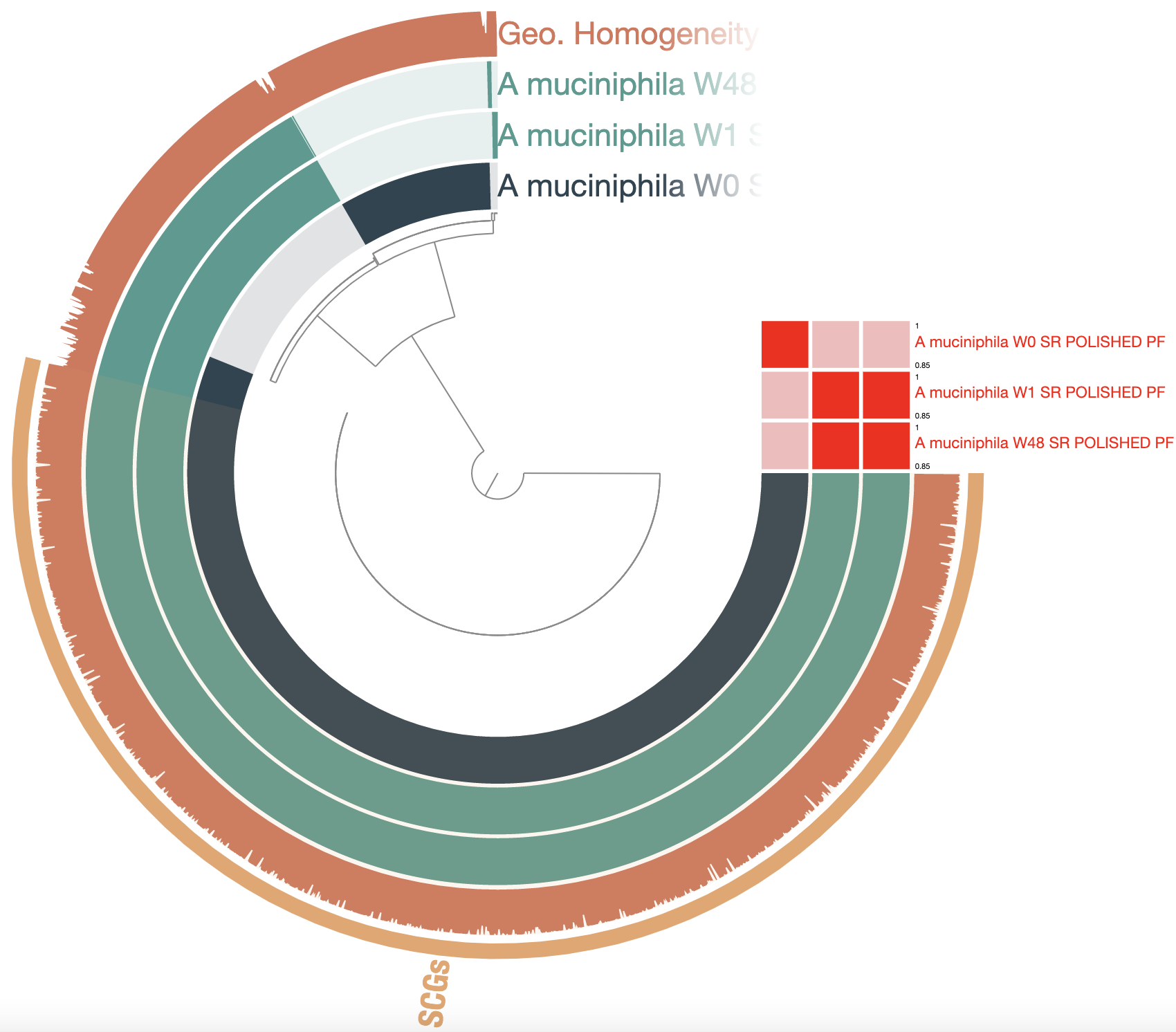
What an improvement overall! Now we only have 15 singleton GCs for W1 and W48, and almost all the core genome is made of single-copy gene cluster. The geometric homogeneity is also very high.
Summary of the polishing/correction strategies for the proovframe preprint:
Now what?
The purpose of this tutorial was to walk you though a real long-read metagenomic analaysis, with a focus on a series of circular genomes reconstructed from the assembly of these metagenomes.
Now that we have our three genomes of Akkermansia muciniphila, we can start to do some real science, depending on your question of interest.
Pangenomics analyis of multiple Akkermansia muciniphila
We have been working with these Akkermansia muciniphila genomes but haven’t looked at their taxonomical assignation yet. We can use anvi’o to estimate the taxonomy of our three corrected genomes:
anvi-estimate-scg-taxonomy -c ANVIO_DATABASES/04_SR_POLISHED_PF/02_CONTIGS/A_muciniphila_W0_SR_POLISHED_PF-contigs.db
anvi-estimate-scg-taxonomy -c ANVIO_DATABASES/04_SR_POLISHED_PF/02_CONTIGS/A_muciniphila_W1_SR_POLISHED_PF-contigs.db
anvi-estimate-scg-taxonomy -c ANVIO_DATABASES/04_SR_POLISHED_PF/02_CONTIGS/A_muciniphila_W48_SR_POLISHED_PF-contigs.db
They are all assigned to the species level, yet W0 differs from W1 & W48 with and ANI around 87%, which is way beyond the commonly used threshold of 95/96% for the species level. To investigate a little bit more the potential level of diversity within the Akkermansia muciniphila species, we can use all the available genomes and assemblies of that species from NCBI.
Get all Akkermansia muciniphila from NCBI
We use ncbi-genome-download to get all Akkermansia muciniphila genomes from NCBI. You can find a more comprehensive tutorial here.
You can run pip install ncbi-genome-download in your anvi’o environment to install the program.
Download all genomes:
ncbi-genome-download bacteria \
                     --assembly-level all \
                     --genus "Akkermansia muciniphila" \
                     --metadata metadata.txt
Then use anvi-script-process-genbank-metadata to generate the fasta files of contigs and a fasta-txt:
anvi-script-process-genbank-metadata -m metadata.txt \
                                     -o NCBI_genomes \
                                     --output-fasta-txt fasta.txt
We have 110 genomes (whole genomes or assembly contigs) to which we added the three genomes W0, W1 and W48. We used the anvi’o pangenomics workflow, but this time on a cluster with more resources to cope with the number of genomes we’re using. We also used fastANI to compute the average nucleotide identity between each pair of genomes.
To visualize the resulting pangenome:
anvi-display-pan -p ANVIO_DATABASES/05_NCBI_GENOMES/Akkermansia_muciniphila_NCBI-PAN.db
Show/hide NCBI _Akkermansia muciniphila_ pangenome

Our genomes of interest can be found in the inner circlers (most inner circle for W0, and in light blue for W1 and W48).
You can obviously notice that the ANI based clustering created three (four with W0) clusters with 86/87% ANI between each group. Indeed it has already been noticed that the species Akkermansia muciniphila currently includes members that should be probably considered as separate species (Guo et al. 2017).
Genomes in green represent whole genome from cultivars and they can only be found in the large cluster of Akkermansia muciniphila. Meaning we have a complete genome from a poorly represented clade of Akkermansia.
Compare pre-FMT and post-FMT Akkermansia muciniphila
How was the donor’s Akkermansia muciniphila able to out-compete a pre-existing population in a recipient’s gut? That is a key question to better understand how microbial populations colonize the human gut.
We saw that the core genome of our three Akkermansia muciniphila is quite large, and will not be informative for us. We need to investigate the content of the accessory genome to generate hypothesis as to how and why the donor’s population replaced the recipient’s one.
Let’s start the interactive interface again, with the most polished/corrected genomes:
anvi-display-pan -g ANVIO_DATABASES/04_SR_POLISHED_PF/03_PAN/A_muciniphila-GENOMES.db \
                 -p ANVIO_DATABASES/04_SR_POLISHED_PF/03_PAN/A_muciniphila-PAN.db
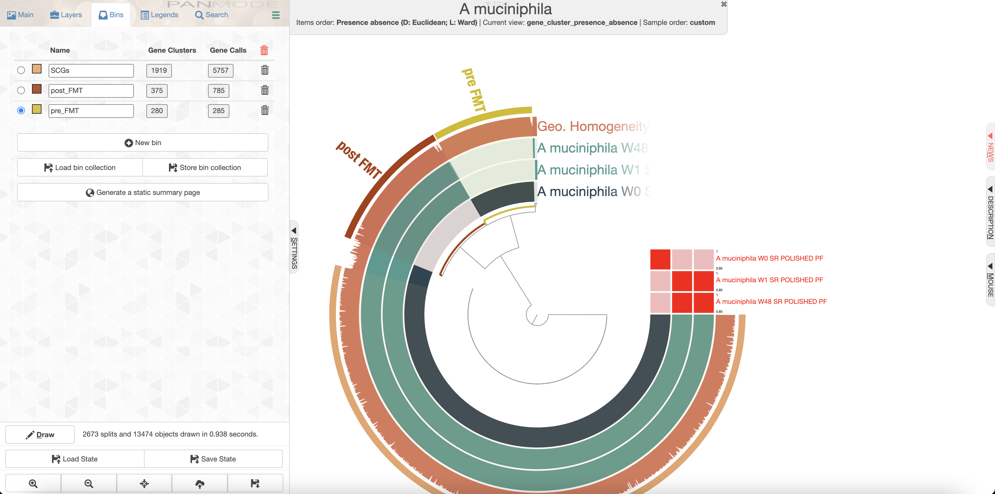
We’ll create bins for the accessory genomes which should look like this:
Now we can use anvi-summarize to generate a table with all the gene calls, their functional annotations and their respective bins.
anvi-summarize -g ANVIO_DATABASES/04_SR_POLISHED_PF/03_PAN/A_muciniphila-GENOMES.db \
               -p ANVIO_DATABASES/04_SR_POLISHED_PF/03_PAN/A_muciniphila-PAN.db \
               -C default \
               -o SUMMARY_PANGENOME
Now let’s have a look at the summary table:
cd SUMMARY_PANGENOME
gunzip A_muciniphila_gene_clusters_summary.txt.gz
Extract the gene annotations (COGs) from the pre_FMT collection (W0):
awk -F "\t" '{if($3=="pre_FMT" && $4~/W0/){print $24 "\t" $18}}' A_muciniphila_gene_clusters_summary.txt | sort | uniq -c > pre_FMT_functions.txt
And also for post_FMT (focusing on W1, but it is the same for W48):
awk -F "\t" '{if($3=="post_FMT" && $4~/W1/){print $24 "\t" $18}}' A_muciniphila_gene_clusters_summary.txt | sort | uniq -c > post_FMT_functions.txt
One should be careful when looking at the functions found in an accessory genome as there might be redundant functions in the core genome. In this case, there was an iron III transport system that was only found in the post-FMT Akkermansia muciniphila. This feature, in addition to the presence of putative antibiotic resistance genes are probably the most interesting functions that could explain how the donor’s Akkermansia muciniphila was able to overcome the recipient’s population.