Refining Metagenome-Assembled Genomes
Table of Contents
- Introduction
- Taking a first look at your MAG
- Refining using sequence composition and differential coverage
- Scrutinizing MAGs with various methods
- Blasting HMM hits of single-copy core genes
- Phylogeny with some genomes from NCBI
- Comparing pagenomes using refined and unrefined MAGs
- Summary
- Reproducible workflow
- Setting the stage
- Generating a merged FASTA file for the MAGs
- Generating a collection file for the merged FASTA file
- Running the anvi’o metagenomic workflow
- Taking a look at the output files
- Getting finalized views and statistics for the genomes we refined
- Importing default collections
- Import default states
- Generating summaries for the refined MAGs
- Getting the completion and redundancy statistics
- Computing phylogeny
- Computing the pangenomes
Summary
The purpose of this tutorial is to discuss key aspects of the refinement of meatgenome-assembled genomes (MAGs). We will use anvi’o to demonstrate each step, however, these principles are independent of anvi’o and can be investigated through other means.
The tutorial includes recommendations to streamline your examination of MAGs, and provides a practical workflow with examples that clarify details of the anvi’o interactive interface. The tutorial broadly covers the following topics:
- Using sequence composition and differential coverage to investigate MAGs in detail to identify contamination (including some tips on using the anvi’o interactive interface effectively).
- Using phylogenomics to investigate refinement efforts in an evolutionary context.
- Using pangenomics to study differences between refined and original MAGs.
While these approaches are independent of any particular dataset or study, to demonstrate their efficacy using a real-world dataset, we will use some of the key MAGs published by Espinoza et al. using the public data the authors kindly provided. At the end of this document you will find a full description of the commands we run to reproduce all steps we run on Esponoza et al. data.
The doi:10.1128/mBio.00725-19 serves the open-access peer-reviewed study described in this document.
Refined MAGs
In addition to demonstrate a step-by-step MAG refinement, we wish to contribute to Espinoza et al.’s study by reporting cleaned verisons of some of their key MAGs that will likely be of great interest to the oral microbiome community due to their originality. The following list reports the FASTA files for the refined Espinoza et al. MAGs that belong to candidate phyla radiation:
- Gracilibacteria (formerly GN02): GN02 MAG.IV.B.1 and GN02 MAG.IV.B.2 (refined from Espinoza et al. MAG IV.B).
- Saccharibacteria (formerly TM7): TM7 MAG.III.A.1 and TM7 MAG.III.A.2 (refined from Espinoza et al. MAG III.A); TM7 MAG III.B.1 (refined from Espinoza et al. MAG III.B). TM7 MAG.III.C.1 (refined from Espinoza et al. MAG III.C).
- Absconditabacteria (formerly SR1): SR1 MAG.IV.A.1 and SR1 MAG.IV.A.2 (refined from Espinoza et al. MAG IV.A; Note: MAG IV.A was annotated as GN2 although a phylogenomic analysis using ribosomal proteins affiliates it with SR1).
If you have any questions, please feel free to leave a comment down below, send an e-mail to us, or get in touch with other anvians through Disord:

Introduction
So you’ve constructed MAGs, and would like to see if there are opportunities for refinement. Great. This tutorial will walk you through an example. We will demonstrate steps that we commonly take to manually refine MAGs we report. Even if refinement of every MAG is not possible, as you will see this is a labor-intensive process, refining critical MAGs may help you and others to prevent misleading insights.
We will walk through this analysis using a specific set of genomes and metagenomes, but you can simply replace these data with yours and follow the same workflow. All you need is this: one or more FASTA files and one or more metagenomes.
If you don’t have your own data to analyze, but still wish to follow the step by step instructions, you can find detailed instructions below to simply download the data we used in this tutorial.
One more thing, througout this blogpost you will encounter sections that look like the one below. These contain extra practical information about working with the anvi’o interactive interface:
Show/Hide Example for expandable practical tips
Feel free to skip these, if you just want to focus on the general discussion of refining MAGs and not interested in the anvi’o interactive interface :-)
Taking a first look at your MAG
At this point in the tutorial, we assume that you have an anvi’o profile database and a contigs database for each MAG you wish to analyze. These are standard file formats anvi’o use to store and read data after processing your FASTA files and your read recruitment results. Generating these files are fairly straightforward and they immediately lend themselves to a myriad of other types of analyses beyond refining your MAGs. You can refer to the instructions at the bottom of this post if you wish to get to this point with FASTA files for your own MAGs and metagenomes from which you recovered them.
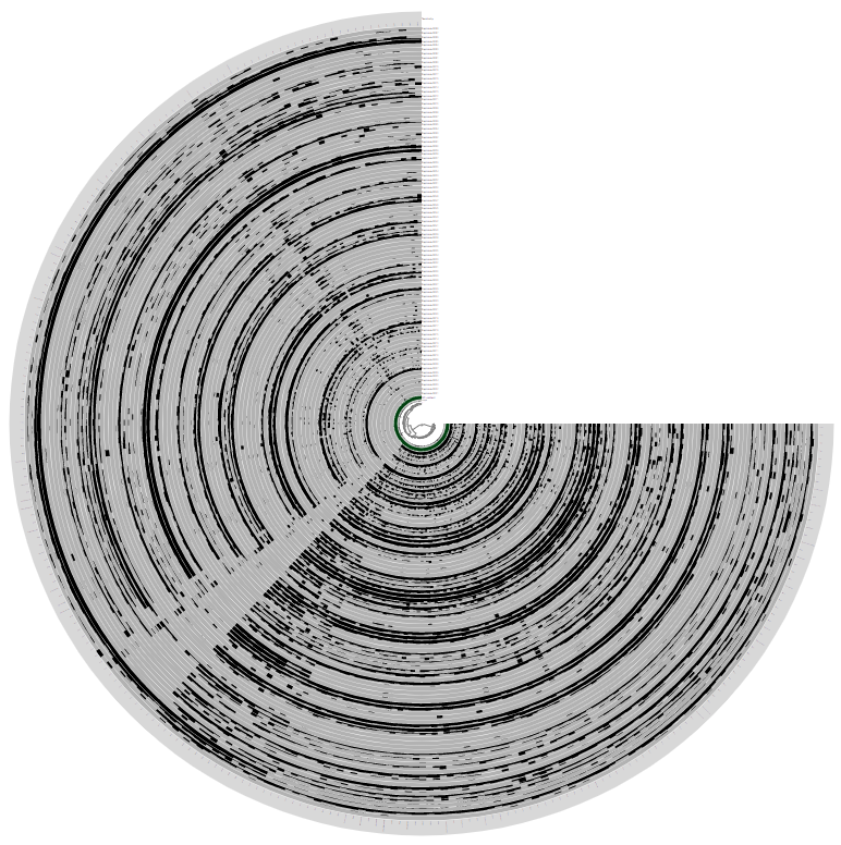
The first step is to take a look at the MAG in the interactive interface using the anvi’o profile and contigs databases. Here we used anvi’o split profiles to manually refine each MAG (generation of which is explained at the end of this post). Here is an example way to initiate the interactive interface for one of those:
anvi-interactive -p 07_SPLIT/GN02_MAG_IV_B/PROFILE.db \
                 -c 07_SPLIT/GN02_MAG_IV_B/CONTIGS.db
Which should give you something that looks like this:
If this is the first time you are seeing an anvi’o interactive interface, we have a separate tutorial here that describes visualization capabilites of anvi’o intearctive interface that may help you orient yourself a little. In addition to that, here we have an extensive tutorial on metagenomic binning that may help you get familiar with some of the anvi’o vocabulary.
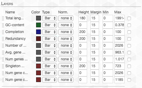
Briefly, every layer in this display is one of the metagenomes, and each item shown here is one of the contigs in this MAG. Data points by default show the mean coverage of a given contig in a given metagenome, but that view can be changed to other things.
There are 88 metagenomes in Espinoza et al. study, hence there are 88 layers in this display. Because we have many metagenomes, the dendrogram in the middle appears too small to make accurate selections of branches. So the first thing we will do is make it bigger.
Show/Hide Changing the radius of the central dendrogram
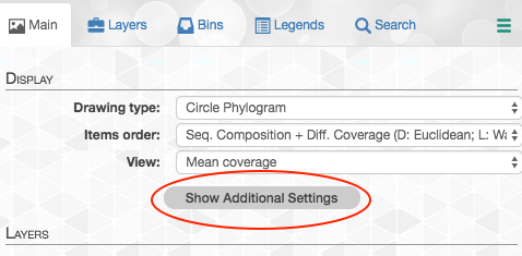
First click on the “Show Additional Settings” button:
And now we can set the radius (here we chose 15,000):

And once we hit “Draw” (or use “d” as a keyboard shortcut), we get this:
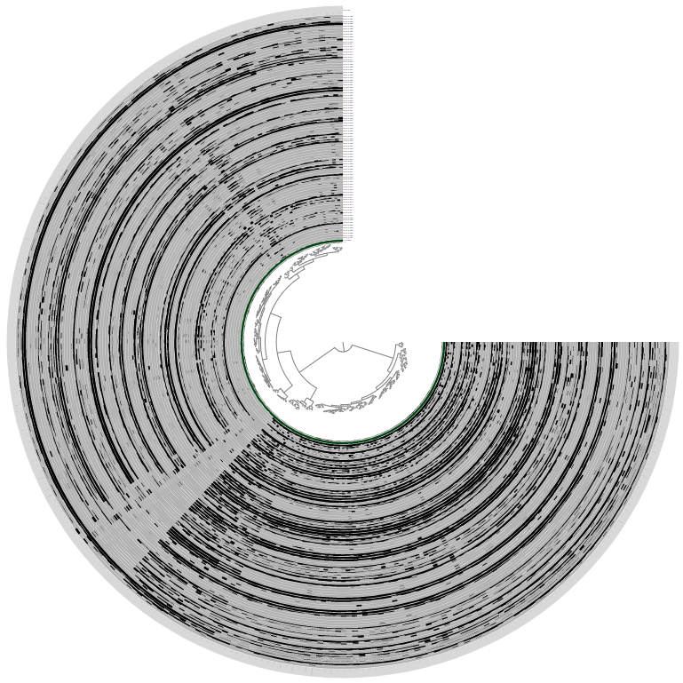
Looks much better. We can already see some interesting patterns, but before we dig into those, let’s examine some general stats regarding these splits in the anvi’o interactive interface.
Show/Hide Examining stats for bins in the interactive interface
To get to see some stats for these splits, we first choose all the splits in this MAG. When you click with the left click on any of the branches in the center dendrogram, it will choose all the items under that part of the tree and add them into a ‘bin’.
You can then move to the “Bins” tab (top left), you can see some real-time stats regarding your MAG:

Once you click the “Bins” tab and you choose all the splits (just choosing the two branches that come out of the root should do it), your interface should look like this:
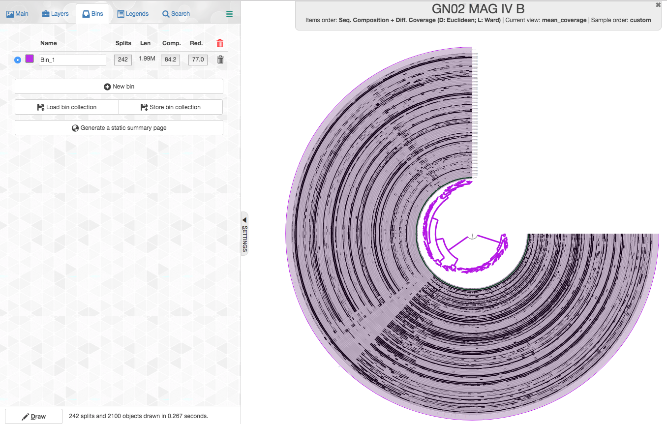
Let’s review what we see:
- Splits: anvi’o splits long contigs into splits of a maximum of 20,000 nucleotides (this is the default, but the number could be modified in
anvi-gen-contigs-database). Here we have 313 splits. - Len: the total length of all the splits (contigs) in your MAG, which in this case is 1.99Mbp. This is already suspicious since other GN02 genomes are much smaller (closer to 1-1.2Mbpa).
- Comp.: completion based on a collection of single-copy core genes. anvi’o has a certain heuristic to determine the domain (bacteria/archea/eukaryota) of the MAG and it would use a dedicated collection of single-copy core genes accordingly. The estimated completion is 84.2%, which would actually be typical to a highly complete member of the CPR.
- Red.: redundancy of single-copy core genes, which is estimated to be 77%.
We can see that this bin has very high redundancy of single-copy core genes. This is a very strong indication that this bin is highly contaminated. In fact, recent guidelines set 10% as the highest redundancy that is appropriate to report for a MAG, with which we agree.
While high redundancy of single-copy core genes is a good predictor of contamination, the lack of redundancy is not an absolute predictor of the lack of contamination. Read Veronika Klevenson’s “Notes on genome refinement with anvi’o”.
We can click on the redundancy number and see which specific genes are redundant:
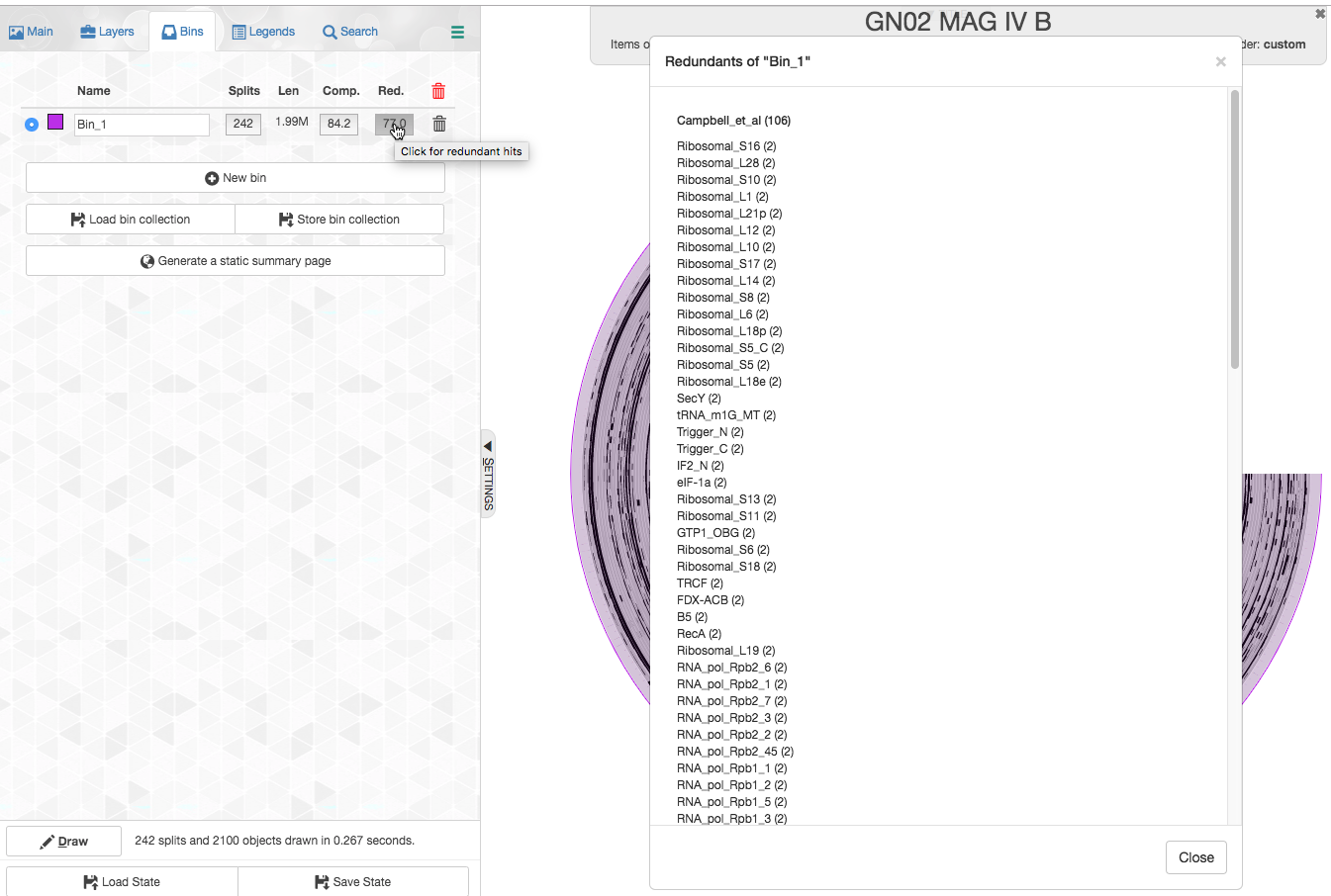
Let’s look for example which splits contain the redundant copies of Ribosomal_S16:
Show/Hide Highlighting redundant single-copy core genes
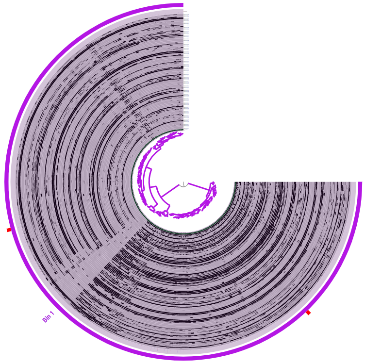
Moreover, if we click on a specific gene name, anvi’o will highlight with a red mark the splits in which the gene occurs. Let’s click on the first one (Ribosomal_S16):
In order to see the highlights better, let’s first go back to the “Main” tab (top right of screen), and set some parameters for “Selections”. It will make our selections and highlights much more visible:

And now the interactive interface should look like this:
In order to get an idea of what taxa these copies of Ribosomal protein S16 represent, we can BLAST the splits in which these genes are found against the NCBI’s nr database.
Show/Hide Getting sequences for splits
This could be done from the interactive interface easily. We simply right click on one of these splits, and then a menu such as in the screenshot below will appear:
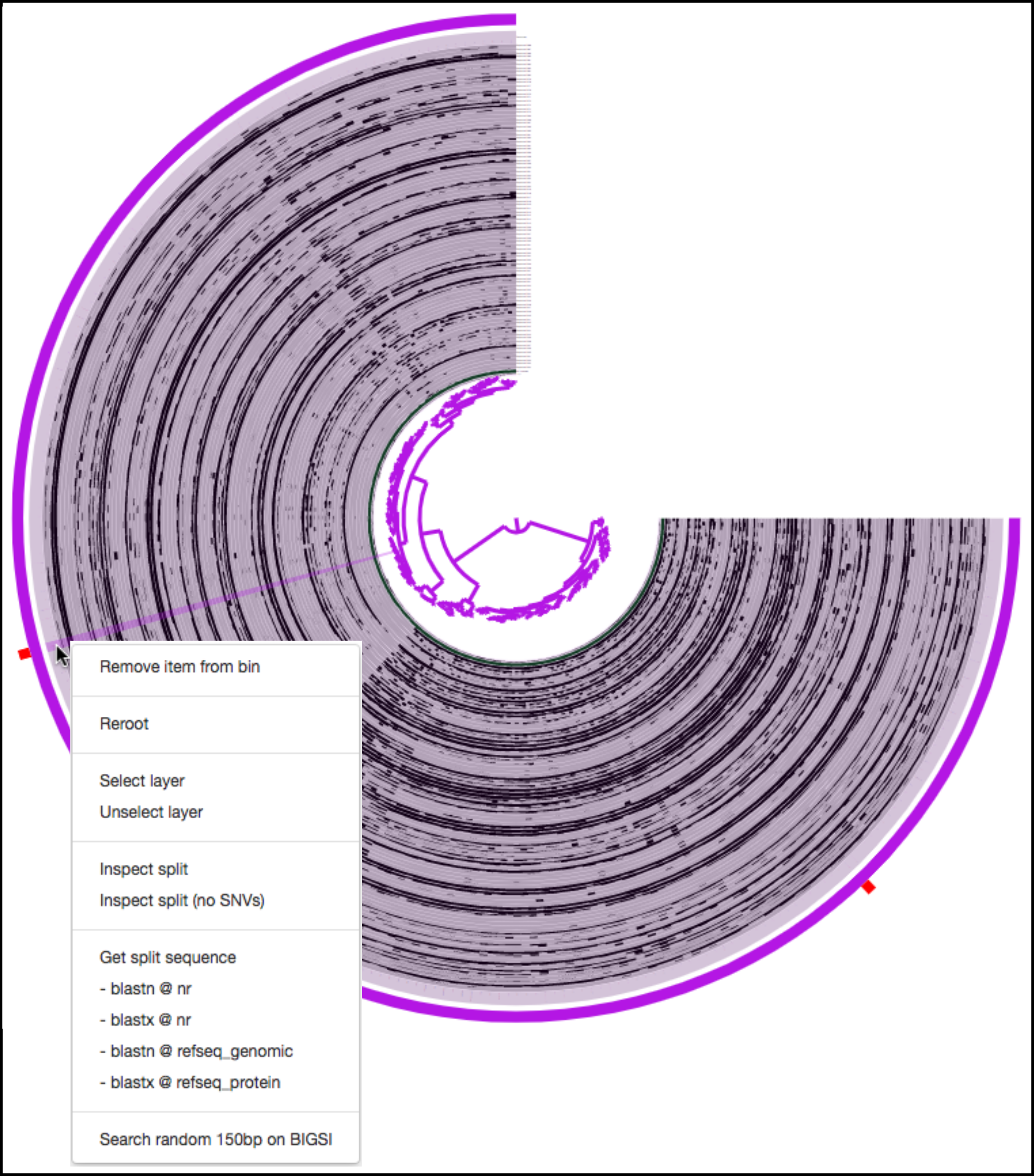
Now, we can either choose one of the “blast” options from below, but I like to choose “Get split sequence”. Choosing this option will prompt the following screen:
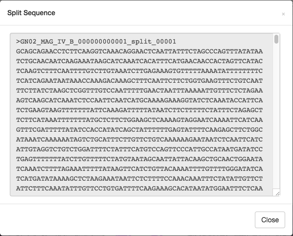
If we click on the sequence inside this window, then the sequence will be highlighted and we can copy and paste it into balstx and run the blastx search (blastx accepts nucleotide sequences as input, translates open reading frames to amino acid sequences and searches NCBI’s protein sequences database). Depending on the length and content of a split this could be very fast or very slow. In this case it took about 10 minutes to get a result.
We can repeat this process for the other split that contains a copy of Ribosomal protein S16.
Here are the screenshot of the top two hits on NCBI for one of the splits:

The top hit is to the original MAG published by Espinoza et al. so that is of no interest. The second hit is to a Gracilibacteria genome HOT-871 from a study by Jouline et al..
And here are the top hits for the second split:

Again the top hit is to the original genome from Espinoza et al., but the second hit is to a different Gracilibacteria genome HOT-872 which is also from the study by Jouline et al..
So the two copies of the genes likely both represent populations from the candidate phylum Gracilibacteria (formerly GN02), but blast tells us that they hit different genomes. In addition, we can see that these copies of Ribosomal protein S16 occur in two sides of the figure that represent very distinct sections of the organizing dendrogram in the middle. This is a good sign that tells us refinement is going to be easy and effective.
Ok, so now it is time to talk about that dendrogram in the middle.
Refining using sequence composition and differential coverage
The dendrogram in the middle organizes the items of the interactive interface. In this case the items represent splits.
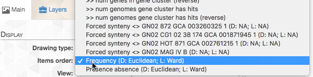
If you click on the “Items order”, you can choose from multiple options of items orders:
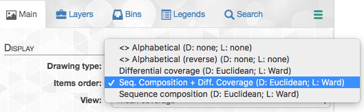
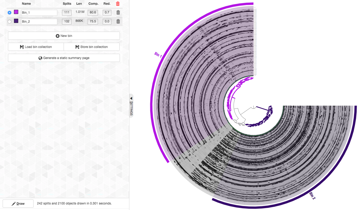
You can read more about each of these options in the “Infant Gut Tutorial”. By default, items are organized by a metric that uses both sequence composition and differential coverage. We can see that the dendrogram separates into two major clusters that appear to have distinct differential coverages. Let’s make two bins with these distinct clusters:
Pro tip. On Mac, you can use ⌘ + mouse click on a branch to store it in a new bin.
Pro tip. Right click on a branch removes it from whatever bin it was in.
Sad tip. The anvi’o interactive interface does not have a CTRL-Z.
We can see that these two clusters correspond to two genomes with very high completion and very low redundancy (C/R of 80.6%/0.7% for Bin_1 and 75.5%/0% for Bin_2). As we show below, these genomes belong to the candidate phylum Gracilibacteria (formerly GN02), a member of the Candidate Phyla Radiation (CPR), and hence this completion estimation is an underestimation.
So here we are, we took just a few fairly easy steps and we have already improved these genomes A LOT!
But what about those splits that now belong to no bin? We will start with the cluster shown below:

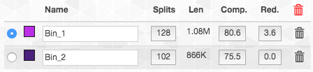
The coverage pattern tells us that these splits are covered in samples in which either of these populations occur, so these are likely largely “shared” sequences of these populations, i.e. sequences that recruit short reads from both of these populations. So let’s check what happens when we add these splits to each of the bins
This is what happens if we add it to bin1:
In contrast, this is what happens if we add it to bin2:

So the completion and redundancy estimates tell us that these splits fit better in bin2 than in bin1. Hence that is where we decided to put them. These type of choices are common to manual refinement and are never easy to make. The best course of action is to continue to scrutinize the MAGs, as we will discuss below. But it is also important to remember that getting a “perfect” MAG could be very difficult, and in some cases may be impossible. It is important to go down the road, but also to remember to not get lost.
What about the remaining splits? When we add these splits to either of the bins, they don’t contribute to completion nor to redundancy. The coverage shows that these are sequences that are largely missing from both of these populations, and hence we decided to not add these to either of the bins.
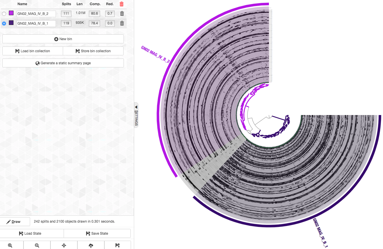
So here are the final bins (now with nicer names too. You can change the names of a bin by clicking on it in the “Bins” tab):
We repeated this refinement process for the rest of the Espinoza et al. CPR bins (GN02 MAG IV.A TM7 MAG III.A TM7 MAG III.B TM7 MAG III.C), to get refined MAGs (to get these refinement results go to the section below).
But we don’t stop here. Next, we will discuss the various ways in which we scrutinize our MAGs.
Scrutinizing MAGs with various methods
Even though metagenome-assembled genomes (MAGs) are key to discover unusual things, usually, when you see a MAG that is unusual, your first assumption should be that it is due to contamination.
In this section we discuss how we use various methods, such as phylogenomics, pangenomics, average nucleotide identity (ANI), taxonomy of genes and genomes, and anything else we can put our hands on to try to identify contamination in MAGs.
Blasting HMM hits of single-copy core genes
One step we often take when working on MAGs is to export the amino-acid sequences of all the Campbell et al. HMM hits and blast these on the NCBI nr database.
In this case, we already blasted a split from each of the refined MAGs (see above), and so we skipped this step, but I still wanted to put this note here in case you want to do it.
To export these sequenes for our case we run:
anvi-get-sequences-for-hmm-hits -c 07_SPLIT/GN02_MAG_IV_B/CONTIGS.db \
                                -p 07_SPLIT/GN02_MAG_IV_B/PROFILE.db \
                                -C default \
                                -b GN02_MAG_IV_B_1 \
                                -o GN02_MAG_IV_B_1-campbell-et-al.fa
We can use the output FASTA file to blast on NCBI (which we didn’t, but you can).
Phylogeny with some genomes from NCBI
Earlier we blasted sequences from each of the refined MAGs, which gave us the idea that these MAGs belong to Candidatus Gracilibacteria. To gain more confidence in this taxonomic assignment we will compute a phylogenetic tree. In addition, a phylogenetic analysis is a good way to see things that seem out of the ordinary. For example, if your MAG branches far away from other genomes, it could be that there is nothing closely related to it on NCBI (yay for you!), but often it could mean that the sequences you used for phylogeny originate from various populations, namely, your MAG is contaminated (boo!).
We downloaded some genomes that belong to each of the phyla that these CPR MAGs belong to (we included the two Gracilibateria genomes from Jouline et al. that we mentioned before).
To read about how we usually go about getting genomes for such phylogenomic and pangenomic analyses, you can refer to this blogpost
To see the details of how we generated this phylogeny you can refer to the section below.
Let’s take a look at the phylogeny:
anvi-interactive --manual \
                 -p 09_PHYLOGENOMICS_WITH_FIRMICUTES/PHYLOGENY-MANUAL-PROFILE.db \
                 -t 09_PHYLOGENOMICS_WITH_FIRMICUTES/ESPINOZA_CPR_MAGS-proteins_GAPS_REMOVED.fa.contree
Show/Hide Changing the "drawing type" in anvi'o
Phylogenies often look better when viewd in a phylogram instead of a circular phylogram. This is what we do to change the “Drawing type” to “Phylogram”:

We also made some manual selections to highlight the MAGs we refined and we get:
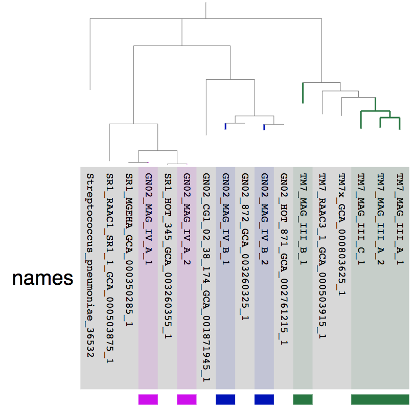
The fact that the MAGs we refined from the Espinoza et al. MAG IV.A and MAG IV.B each have a very closely related genome from an independent study is a good sign that these are good quality genomes. On the other hand, lack of closely related genomes for the TM7 genomes doesn’t necessarily mean anything.
Comparing pagenomes using refined and unrefined MAGs
To highlight some of the differences between the refined and unrefined MAGs, we computed a pangenome using the anvi’o pangenomic workflow for each of the three phyla (TM7, GN02, and SR1) using the genomes we used for the phylogeny above.
Here we will only present and discuss the results for MAG IV.B that we discussed in detail above.
Let’s take a look at the pangenome:
anvi-display-pan -p 10_PAN/GN02_UNREFINED/GN02_UNREFINED-PAN.db \
                 -g 10_PAN/GN02-UNREFINED-GENOMES.db
Ok, there is a lot here, and if you want to learn about all the wonderful information that is presented here, you should refer to the anvi’o pangenomics tutorial. We really recommend that you take a look, because there are a lot of things you can learn from a pangenome.
In our case we will focus on just one thing: the single-copy core gene clusters (“SCG Clusters” or simply “SCGs”). The SCGs are gene clusters that occur with a single copy in ALL genomes in the pangenome. Similar to how we use the redundancy of single copy core genes from an HMM collection to estimate contamination, we can also use SCGs as a similar indicator as we show below. The figure above contains concentric circular sections to represent each of the four genomes we used for computing the pangenomes. In addition, there are 5 additional concentric layers, but we are only interested in the one that is labeled “SCG Clusters”.
So we will remove the rest of the layers from the iterface, and change a few more things to make it easier to examine the SCGs.
Show/Hide Modifying the interactive interface for the pangenome
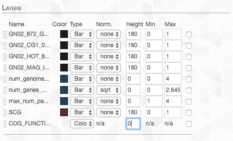
In order to remove the layers that are currently of no interest to us, we go to the “Main” tab and set the “Height” to zero for each layer we don’t want:
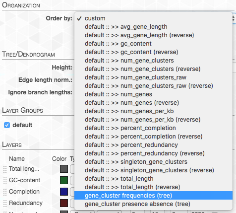
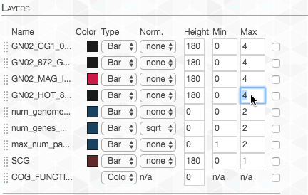
On the right top corner of the figure above we also have some additional statistics for each of the four genomes. We can change what is presented by navigating to the “Layers” tab. The first thing we do, is to change the “Order by” in order to organize the genomes according to “gene_cluster frequencies”:
This will change the order of layers so that genomes that contain similar gene clusters will be closer together (it will also add a tree that describes this clustering).
We can also change which information is shown. I changed the values to these:
In addition, in the “Main” tab, we can change the organization of the gene-clusters (namely the organizing dendrogram at the middle of the figure):
By default, the data is shown as presence/absence of each gene cluster in each genome, but in this case we want to see how many copies of each gene cluster are in each genome. So we change the “View”:

We want the maximum value to be the same for each layer, so we adjust the “Max”:
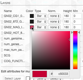
Lastly, I changed the color of the layer representing our genome-of-interest to highlight it:
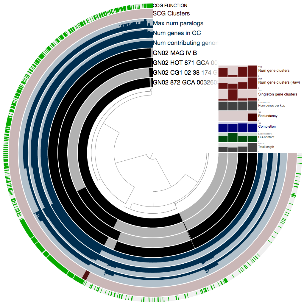
And now we can take another look:
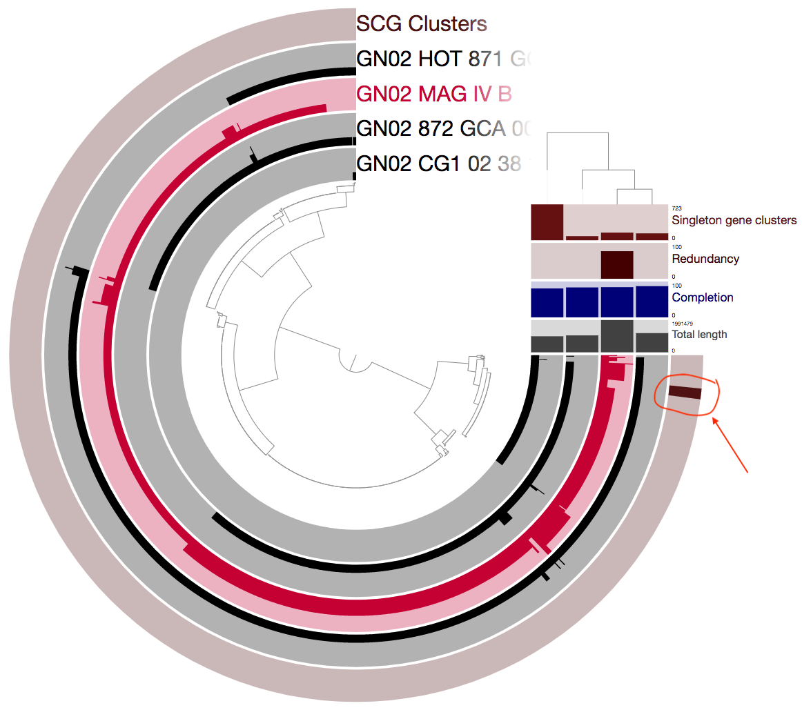
I encircled and added an arrow above to emphesize the single-copy core gene clusters (SCGs). The SCGs are important because we can use these for many things. For example, these could be great to use for phylogeny. But in our case the fact that there are only 8 such gene clusters is a pretty alarming sign that something is wrong. A closer examination of the figure above reveals that there are many gene clusters that appear as single-copy in the other three genomes, but as multi-copy in MAG IV.B.
Let’s now take a look at the pangenome using the refined genomes:
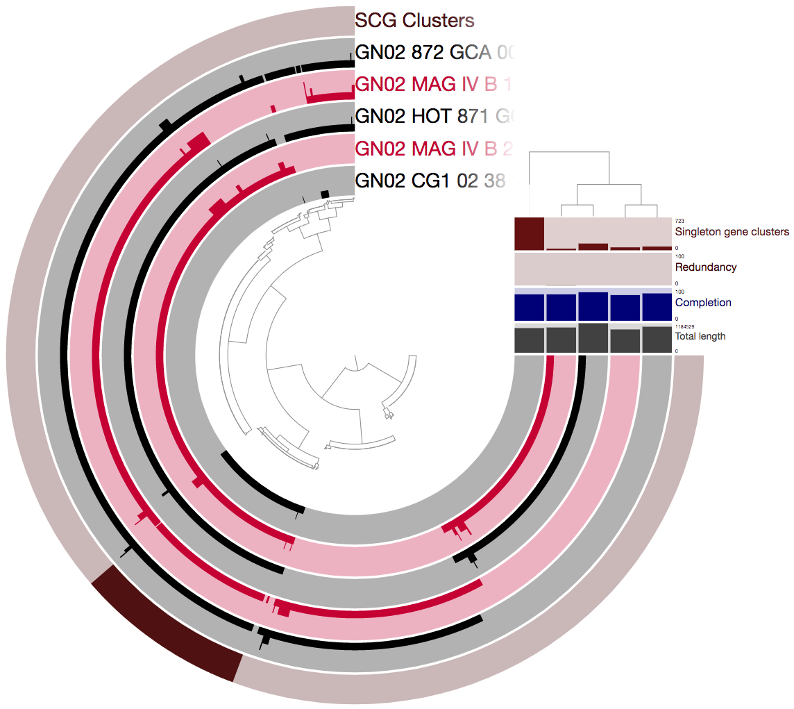
We can see that there are now many more SCGs (there are 128 such gene clusters, a 1,600% increase compared to earlier).
Summary
Here we presented steps you can take if you want to examine some genomes using metagenomes.
There are many more things that could be done, and we will try to extend this tutorial in the future.
The bottom line is that we strongly encourage to explore MAGs in various ways.
Reproducible workflow
Here you will find all the computational steps that are required to get the results we discussed above.
Setting the stage
This section explains how to download the metagenomes and MAGs from the original study by Espinoza et al. Downloading this data would allow you to follow this post step by step and get the final results we got. Alternatively, you can skip this part, and apply the approach we describe to your own data.
Downloading the Espinoza et al. metagenomes
You can download raw Illumina paired-end seqeuncing data files for the 88 supragingival plaque samples into your work directory the following way:
curl -L -O http://merenlab.org/data/refining-mags/files/SRR_list.txt

for SRR_accession in `cat SRR_list.txt`; do
    fastq-dump --outdir 01_RAW_FASTQ \
               --gzip \
               --skip-technical  \
               --readids \
               --read-filter pass \
               --dumpbase \
               --split-3 \
               --clip \
               $SRR_accession
done
Once the download is finished, you should have 196 FASTQ files in your 01_RAW_FASTQ directory, representing the paired-end reads of 88 metagenomes.
Downloading key MAGs from Espinoza et al.
In our reanalysis we only focused on some of the key MAGs that represented understudied lineages in the oral cavity. You can download these FASTA files from the NCBI GenBank in the following way:
mkdir -p 01_FASTA

# TM7_MAG_III_A (bin_8)
curl -L ftp://ftp.ncbi.nlm.nih.gov/genomes/all/GCA/003/638/965/GCA_003638965.1_ASM363896v1/GCA_003638965.1_ASM363896v1_genomic.fna.gz \
    -o 01_FASTA/TM7_MAG_III_A.fa.gz

# TM7_MAG_III_B (bin_9)
curl -L ftp://ftp.ncbi.nlm.nih.gov/genomes/all/GCA/003/638/935/GCA_003638935.1_ASM363893v1/GCA_003638935.1_ASM363893v1_genomic.fna.gz \
    -o 01_FASTA/TM7_MAG_III_B.fa.gz

# TM7_MAG_III_C (bin_10)
curl -L ftp://ftp.ncbi.nlm.nih.gov/genomes/all/GCA/003/638/915/GCA_003638915.1_ASM363891v1/GCA_003638915.1_ASM363891v1_genomic.fna.gz \
    -o 01_FASTA/TM7_MAG_III_C.fa.gz

# GN02_MAG_IV_A (bin_15)
curl -L ftp://ftp.ncbi.nlm.nih.gov/genomes/all/GCA/003/638/815/GCA_003638815.1_ASM363881v1/GCA_003638815.1_ASM363881v1_genomic.fna.gz \
     -o 01_FASTA/GN02_MAG_IV_A.fa.gz

# GN02_MAG_IV_B (bin_16)
curl -L ftp://ftp.ncbi.nlm.nih.gov/genomes/all/GCA/003/638/805/GCA_003638805.1_ASM363880v1/GCA_003638805.1_ASM363880v1_genomic.fna.gz \
     -o 01_FASTA/GN02_MAG_IV_B.fa.gz
Before we go into refining we wish to take a look at the individual fasta files. To do that we use the contigs database, which allows us to annotate each fasta file and compute some basic statistics such as redundancy and completion based on single-copy core genes.
To sreamline the contigs database creation and annotation, we used anvi-run-workflow. This is a tool that is meant to help streamline the analysis steps and make things fully reproducible. For more details regarding anvi-run-workflow and other anvi’o worfklows please read this tutorial).
Generating a merged FASTA file for the MAGs
You can skip this section if you are working with your own FASTA file(s) and you do not wish to merge them.
When working with multiple FASTA files you can choose between analysing each separately or concatinating them into a single FASTA file. The main advantage of working with a single FASTA file in our case is that mapping short reads to a single large FASTA file is much faster than mapping reads to multiple smaller files. Depending on your specific data you should decide what’s better for your case. In this case we chose to use a single merged FASTA file since the MAGs that we examined originated from an assembly that was done with the exact metagenomes that we use here. all the steps that are done here could be done with multiple fasta files (and hence multiple contigs databases) in the same manner. To make things go a little faster, we combined all MAGs into a single FASTA file (so the mapping and profiling steps could be streamlined).
In order to create a merged FASTA file, we first wish to rename the headers in each FASTA file to have names that are meaningful (so that we know for each contig, what genome it originated from) and also names that are acceptable for anvi’o (i.e. ASCII and ‘_’). For that, we used the following text file, ESPINOZA-MAGS-FASTA.txt, which is in the format of a fasta_txt file as accepted by anvi-run-workflow.
You can download this file by running the following command:
curl -L -O http://merenlab.org/data/refining-mags/files/ESPINOZA-MAGS-FASTA.txt
Here is a look into this file:
$ column -t ESPINOZA-MAGS-FASTA.txt
name                     path
TM7_MAG_III_A            01_FASTA/TM7_MAG_III_A.fa.gz
TM7_MAG_III_B            01_FASTA/TM7_MAG_III_B.fa.gz
TM7_MAG_III_C            01_FASTA/TM7_MAG_III_C.fa.gz
GN02_MAG_IV_A            01_FASTA/GN02_MAG_IV_A.fa.gz
GN02_MAG_IV_B            01_FASTA/GN02_MAG_IV_B.fa.gz
In addition, we used the following config file CONTIGS-CONFIG.json:
{
    "anvi_run_ncbi_cogs": {
        "run": false
    },
    "fasta_txt": "ESPINOZA-MAGS-FASTA.txt"
}
You can download this file by running the following command:
curl -L -O http://merenlab.org/data/refining-mags/files/CONTIGS-CONFIG.json
We used the contigs workflow to just re-format these FASTA files:
anvi-run-workflow -w contigs \
                  -c CONTIGS-CONFIG.json \
                  --additional-params \
                    --until anvi_script_reformat_fasta_prefix_only
This command will extract the raw FASTA files into temporary FASTA files, reformat these, and delete the extracted temporary fasta files.
At his point we can merge the fasta files into one file:
cat 01_FASTA/*/*-contigs-prefix-formatted-only.fa \
					               > 01_FASTA/ESPINOZA-MAGS-MERGED.fa
And we create a new fasta_txt file that we named ESPINOZA-MERGED-FASTA.txt:
echo -e "name\tpath" > ESPINOZA-MERGED-FASTA.txt
echo -e "ESPINOZA\t01_FASTA/ESPINOZA-MAGS-MERGED.fa" >> ESPINOZA-MERGED-FASTA.txt
It should look like this:
$ column -t ESPINOZA-MERGED-FASTA.txt
name      path
ESPINOZA  01_FASTA/ESPINOZA-MAGS-MERGED.fa
Generating a collection file for the merged FASTA file
This step is also necessary only if you are working with a merged FASTA file. A collection is what anvi’o uses to know which contig is associated with which genome.
We generated a collection file that we could later use to import into the anvi’o merged profile database.
In order to generate this file, we used the following python script: gen-collection-for-merged-fasta.py, which you can download in the following way:
curl -L -O https://gist.githubusercontent.com/ShaiberAlon/23fc13ed56e02854bee42773672832a5/raw/3322cf23effe3325b9f8d97615f0b5af212b2fc2/gen-collection-for-merged-fasta.py
This script takes a fasta_txt file as input and generates a collection file where the name of each entry in the fasta_txt file is associated with the names of contigs in the respective FASTA file.
The following BASH one liner will generate a TAB delmited file (which will be our fasta_txt mentioned above) for the newly generated reformated FASTA files:
ls 01_FASTA/*/*.fa | \
    awk 'BEGIN{FS="/"; print "name\tpath"}
              {print $2 "\t" $0}' > ESPINOZA-MAGS-REFORMATTED-FASTA.txt
This is what the contents of this file looks like:
column -t ESPINOZA-MAGS-REFORMATTED-FASTA.txt
name	path
GN02_MAG_IV_A	01_FASTA/GN02_MAG_IV_A/GN02_MAG_IV_A-contigs-prefix-formatted-only.fa
GN02_MAG_IV_B	01_FASTA/GN02_MAG_IV_B/GN02_MAG_IV_B-contigs-prefix-formatted-only.fa
TM7_MAG_III_A	01_FASTA/TM7_MAG_III_A/TM7_MAG_III_A-contigs-prefix-formatted-only.fa
TM7_MAG_III_B	01_FASTA/TM7_MAG_III_B/TM7_MAG_III_B-contigs-prefix-formatted-only.fa
TM7_MAG_III_C	01_FASTA/TM7_MAG_III_C/TM7_MAG_III_C-contigs-prefix-formatted-only.fa
Now we can generate the collection file:
python gen-collection-for-merged-fasta.py -f ESPINOZA-MAGS-REFORMATTED-FASTA.txt \
                                          -o ESPINOZA-MAGS-COLLECTION.txt
Here is a glimpse to the resulting ESPINOZA-MAGS-COLLECTION.txt:
column -t  ESPINOZA-MAGS-COLLECTION.txt | head -n 5
GN02_MAG_IV_A_000000000001  GN02_MAG_IV_A
GN02_MAG_IV_A_000000000002  GN02_MAG_IV_A
GN02_MAG_IV_A_000000000003  GN02_MAG_IV_A
GN02_MAG_IV_A_000000000004  GN02_MAG_IV_A
GN02_MAG_IV_A_000000000005  GN02_MAG_IV_A
Note that every line in this collection file describes which contig name belongs to which genome.
In order to have the snakemake workflow use this collection automatically, and generate a summary and split databases, we need a collections_txt (as is explained in the anvi-run-workflow tutorial).
We named our collections_txt ESPINOZA-COLLECTIONS-FILE.txt.
You can download this file to your work directory:
curl -L -O http://merenlab.org/data/refining-mags/files/ESPINOZA-COLLECTIONS-FILE.txt
 $ column -t ESPINOZA-COLLECTIONS-FILE.txt
name       collection_name   collection_file                contigs_mode
ESPINOZA   ORIGINAL_MAGS     ESPINOZA-MAGS-COLLECTION.txt   1
Notice that we set the value in the contigs_mode column to 1, because our collection file ESPINOZA-MAGS-COLLECTION.txt contains names of contigs and not names of splits.
Running the anvi’o metagenomic workflow
The analysis described here utilizes the anvi’o contigs and profile databases. You can refer to the anvi’o metagenomic tutorial to learn more about these databases in a general manner or to this tutorial to see many of the things that you could do using anvi’o. In this post we will assume a basic familiarity of anvi’o. In order to streamline the process of generating and annotating a contigs database and a merged profile database we used the snakemake-based metagenomics workflow. To learn how to use this workflow, you can either follow the steps here or follow the step-by-step process in the anvi’o metagenomic tutorial.
First we will describe all the necesary files for the workflow.
One of the key input files to start the run is the samples.txt. You can downlaod our samples.txt file into your work directory:
curl -L -O http://merenlab.org/data/refining-mags/files/samples.txt
Here is a glimpse at its contents:
$ column -t samples.txt | head -n 5
sample         r1                                       r2
Espinoza_0001  01_RAW_FASTQ/SRR6865436_pass_1.fastq.gz  01_RAW_FASTQ/SRR6865436_pass_2.fastq.gz
Espinoza_0002  01_RAW_FASTQ/SRR6865437_pass_1.fastq.gz  01_RAW_FASTQ/SRR6865437_pass_2.fastq.gz
Espinoza_0003  01_RAW_FASTQ/SRR6865438_pass_1.fastq.gz  01_RAW_FASTQ/SRR6865438_pass_2.fastq.gz
Espinoza_0004  01_RAW_FASTQ/SRR6865439_pass_1.fastq.gz  01_RAW_FASTQ/SRR6865439_pass_2.fastq.gz
We used the following command to generate a ‘default’ config file for the metagenomics workflow,
anvi-run-workflow -w metagenomics \
                  --get-default-config config.json
And edited it to instruct the workflow manager to,
- Generate a contigs database.
- Run anvi-run-hmms.
- Annotate genes with taxonomy using centrifuge.
- Annotate genes with functions using anvi-run-ncbi-cogs.
- Quality filter short reads using illumina-utils.
- Recruit reads from all samples using the merged FASTA file with Bowtie2.
- Profile and merge resulting files using anvi’o.
- Import the collection into the anvi’o merged profile database.
- Summarize the profile database using
anvi-summarize. - Split each bin into an individual contigs and merged profile database using
anvi-split.
You can download our config file ESPINOZA-METAGENOMICS-CONFIG.json into your work directory:
curl -L -O http://merenlab.org/data/refining-mags/files/ESPINOZA-METAGENOMICS-CONFIG.json
The content of which should look like this:
{
    "fasta_txt": "ESPINOZA-MERGED-FASTA.txt",
    "centrifuge": {
        "threads": 2,
        "run": true,
        "db": "/PATH/TO/CENTRIFUGE/Centrifuge-NR/nt/nt"
    },
    "anvi_run_hmms": {
        "run": true,
        "threads": 5
    },
    "anvi_run_ncbi_cogs": {
        "run": true,
        "threads": 5
    },
    "anvi_script_reformat_fasta": {
        "run": false
    },
    "samples_txt": "samples.txt",
    "iu_filter_quality_minoche": {
        "run": true,
        "--ignore-deflines": true
    },
    "gzip_fastqs": {
        "run": true
    },
    "bowtie": {
        "additional_params": "--no-unal",
        "threads": 3
    },
    "samtools_view": {
        "additional_params": "-F 4"
    },
    "anvi_profile": {
        "threads": 3,
        "--sample-name": "{sample}",
        "--overwrite-output-destinations": true,
        "--profile-SCVs": true,
        "--min-contig-length": 0
    },
    "import_percent_of_reads_mapped": {
        "run": true
    },
    "references_mode": true,
    "all_against_all": true,
    "collections_txt": "ESPINOZA-COLLECTIONS-FILE.txt",
    "anvi_summarize": {
        "run": true
    },
    "anvi_split": {
        "run": true
    },
    "output_dirs": {
        "QC_DIR": "02_QC",
        "CONTIGS_DIR": "03_CONTIGS",
        "MAPPING_DIR": "04_MAPPING",
        "PROFILE_DIR": "05_ANVIO_PROFILE",
        "MERGE_DIR": "06_MERGED",
        "SUMMARY_DIR": "08_SUMMARY",
        "SPLIT_PROFILES_DIR": "07_SPLIT",
        "LOGS_DIR": "00_LOGS"
    }
}
Note that in order for this config file to work for you, the path to the centrifuge database must be fixed to match the path on your machine (or simply set centrifuge not to run by setting the “run” parameter to false).
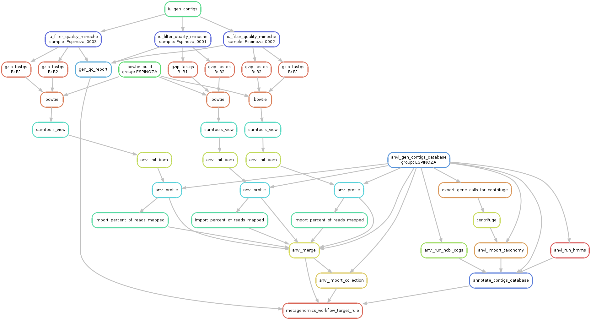
Just to make sure things look alright, we run the following command to generate a visual summary of the workflow:
anvi-run-workflow -w metagenomics \
                  -c ESPINOZA-METAGENOMICS-CONFIG.json \
                  --save-workflow-graph
This original graph with all samples is way too big, but here is a subset of it with only three samples for demonstration purposes:
We finally run this configuration the following way (the --cluster parameters are specific to our server, and will require you to remove that paramter, or format depending on your own server setup):
anvi-run-workflow -w metagenomics \
                  -c ESPINOZA-METAGENOMICS-CONFIG.json \
                  --additional-params \
                      --cluster 'clusterize -log {log} -n {threads}' \
                      --resources nodes=40 \
                      --jobs 10 \
                      --rerun-incomplete
Taking a look at the output files
Successful completion of the anvi’o metagenomic workflow in our case results in 00_LOGS, 02_QC, 03_CONTIGS, 04_MAPPING, 05_ANVIO_PROFILE, 06_MERGED, 07_SPLIT, and 08_SUMMARY folders. The following is the brief summary of the contents of these directories:
-
00_LOGS: Log files for every operation done by the workflow. -
02_QC: Quality-filtered short metagenomic reads and final statistics file (02_QC/qc-report.txt). -
03_CONTIGS: Anvi’o contigs database with COG annotations, centrifuge taxonomy for genes, and HMM hits for single-copy core genes.
$ ls 03_CONTIGS/*db
03_CONTIGS/ESPINOZA-contigs.db
-
04_MAPPING: Bowtie2 read recruitment results for assembly outputs from quality-filtered short metagenomic reads in the form of BAM files. -
05_ANVIO_PROFILE: Anvi’o single profiles for each sample. -
06_MERGED: Anvi’o merged profile databae.
 $ ls -R 06_MERGED
ESPINOZA

06_MERGED/ESPINOZA:
AUXILIARY-DATA.db	PROFILE.db		RUNLOG.txt		collection-import.done
07_SPLIT: Anvi’o split merged profile databases and contigs databases for each bin in the collection.
# For each bin a folder is generated inside 07_SPLIT
ls 07_SPLIT/
GN02_MAG_IV_B			TM7_MAG_III_C
TM7_MAG_III_A			GN02_MAG_IV_A
TM7_MAG_III_B

# Here is an example for one of the split bins:
ls 07_SPLIT/GN02_MAG_IV_A/
AUXILIARY-DATA.db		PROFILE.db			CONTIGS.db
08_SUMMARY: Anvi’o summary for the merged profile database.
Getting finalized views and statistics for the genomes we refined
In this section we describe the process of reproducing our final results from refining the Espinoza et al. MAGs, including the final collections, and a state for the interactive view to show the results in a prettier format.
Importing default collections
You can get the collection files in the following way:
for g in GN02_MAG_IV_A GN02_MAG_IV_B TM7_MAG_III_A TM7_MAG_III_B TM7_MAG_III_C; do
    curl -L -O http://merenlab.org/data/refining-mags/files/$g-default-collection.txt
    curl -L -O http://merenlab.org/data/refining-mags/files/$g-default-collection-info.txt
done
Now we can import these collections:
for g in GN02_MAG_IV_A GN02_MAG_IV_B TM7_MAG_III_A TM7_MAG_III_B TM7_MAG_III_C; do
    anvi-import-collection -c 07_SPLIT/$g/CONTIGS.db \
                           -p 07_SPLIT/$g/PROFILE.db \
                           $g-default-collection.txt \
                           -C default \
                           --bins-info $g-default-collection-info.txt
done
Import default states
You can download the default states in the following way:
for g in GN02_MAG_IV_A GN02_MAG_IV_B TM7_MAG_III_A TM7_MAG_III_B TM7_MAG_III_C; do
    curl -L -O http://merenlab.org/data/refining-mags/files/$g-default-state.json
done
And now we can import these as default states to each profile database:
for g in GN02_MAG_IV_A GN02_MAG_IV_B TM7_MAG_III_A TM7_MAG_III_B TM7_MAG_III_C; do
    anvi-import-state -p 07_SPLIT/$g/PROFILE.db \
                      -n default \
                      -s $g-default-state.json
done
We can run the interactive interface again for the same MAG as earlier:
anvi-interactive -p 07_SPLIT/GN02_MAG_IV_B/PROFILE.db \
                 -c 07_SPLIT/GN02_MAG_IV_B/CONTIGS.db
This is what it should look like now:
Much better :-)
Generating summaries for the refined MAGs
After we finished the refine process, we generated a summary for the collections that we made in each profile database. The purpose of the summary is to have various statistics available for each MAG. In addition, during the summary process FASTA files for each of the refined MAGs are generated.
To generate a summary directory for each profile database we run the following command:
for g in GN02_MAG_IV_A GN02_MAG_IV_B TM7_MAG_III_A TM7_MAG_III_B TM7_MAG_III_C; do
    anvi-summarize -p 07_SPLIT/$g/PROFILE.db \
                      -c 07_SPLIT/$g/CONTIGS.db \
                      -C default \
                      -o 07_SPLIT/$g/SUMMARY
done
Getting the completion and redundancy statistics
In order to compare between the MAGs from the original Espinoza et al publication and our refined MAGs, we examined the completion and redundancy values that were generated using the collection of single-copy core genes from Campbell et al.. These values are included in the bins_summary.txt file inside each SUMMARY folder that was created by anvi-summarize.
The following file includes the completion and redundancy for the original MAGs from Espinoza et al.:
08_SUMMARY/bins_summary.txt
Since TM7 MAG III.A had a particularly high ammount of redundancy, anvi’o wasn’t generating any completion nor redundancy values for it. To bypass this issue, we used the another file that is available in the summary folder:
08_SUMMARY/bin_by_bin/TM7_MAG_III_A/TM7_MAG_III_A-Campbell_et_al-hmm-sequences.txt
This file includes the sequences for all the genes that matched the single-copy core genes from Campbell et al.. We will use the headers of this FASTA file (yes, even though it has a “.txt” suffix, it is a FASTA file), to learn which genes are present in TM7_MAG_III_A and with what copy number:
grep ">" 08_SUMMARY/bin_by_bin/TM7_MAG_III_A/TM7_MAG_III_A-Campbell_et_al-hmm-sequences.txt | \
        sed 's/___/#/' |\
        cut -f 1 -d \# |\
        sed 's/>//' |\
        sort |\
        uniq -c |\
        sed 's/ /\t/g' |\
        rev |\
        cut -f 1,2 |\
        rev > TM7_MAG_III_A-Campbell_et_al-hmm-occurrence.txt
We used the resulting file TM7_MAG_III_A-Campbell_et_al-hmm-occurrence.txt to calculate the completion and redundancy,
which are 84% and 138% respectively.
To generate a table with the details for our refined MAGs, we ran the following command:
head -n 1 07_SPLIT/GN02_MAG_IV_A/SUMMARY/bins_summary.txt > bins_summary_combined.txt

for g in GN02_MAG_IV_A GN02_MAG_IV_B TM7_MAG_III_A TM7_MAG_III_B TM7_MAG_III_C; do
    tail -n +2 07_SPLIT/$g/SUMMARY/bins_summary.txt >> bins_summary_combined.txt
done
Here is what it looks like:
$ column -t bins_summary_combined.txt
bins             taxon       total_length  num_contigs  N50    GC_content          percent_completion  percent_redundancy
GN02_MAG_IV_A_1  None        656014        130          5758   35.675872849368126  52.51798561151079   1.4388489208633093
GN02_MAG_IV_A_2  None        840154        133          7956   38.33379540838725   66.90647482014388   4.316546762589928
GN02_MAG_IV_B_1  None        934609        119          10886  25.10850812472708   78.41726618705036   0.0
GN02_MAG_IV_B_2  None        1012757       109          12715  24.99647116647001   80.57553956834532   0.7194244604316546
TM7_MAG_III_A_1   None        910899        90           14382  47.36125683516097   79.85611510791367   0.0
TM7_MAG_III_A_2   None        445398        99           5809   48.98771936204964   57.55395683453237   0.0
TM7_MAG_III_A_3   None        223971        64           3436   47.962761305917525  22.302158273381295  0.0
TM7_MAG_III_A_4   None        156413        59           2858   46.00378865630705   13.66906474820144   0.7194244604316546
TM7_MAG_III_A_5   None        150222        68           2250   47.400770761670294  15.107913669064748  0.0
TM7_MAG_III_A_6   Candidatus  138985        48           3031   44.220410307583954  10.79136690647482   0.7194244604316546
TM7_MAG_III_B_1   None        534277        233          2931   35.16218616929297   77.6978417266187    5.755395683453237
TM7_MAG_III_C_1   None        772299        440          2432   53.056877029321505  67.62589928057554   4.316546762589928
Computing phylogeny
We downloaded some genomes from the NCBI in order to compute a phylogeny. Below is a table of these genomes (we also include some metadata for each genome).
| name | accession | assembly | reference | title | source | sample_type | study | HOT_designation_according_to_16S_rRNA |
|---|---|---|---|---|---|---|---|---|
| SR1_RAAC1_SR1_1_GCA_000503875_1 | GCA_000503875.1 | ftp://ftp.ncbi.nlm.nih.gov/genomes/all/GCA/000/503/875/GCA_000503875.1_ASM50387v1/GCA_000503875.1_ASM50387v1_genomic.fna.gz | https://mbio.asm.org/content/4/5/e00708-13.short | Small Genomes and Sparse Metabolisms of Sediment-Associated Bacteria from Four Candidate Phyla | Environmental | Environmental | Kantor et al. 2013 | |
| SR1_MGEHA_GCA_000350285_1 | GCA_000350285.1 | ftp://ftp.ncbi.nlm.nih.gov/genomes/all/GCA/000/350/285/GCA_000350285.1_OR1/GCA_000350285.1_OR1_genomic.fna.gz | http://www.pnas.org/cgi/pmidlookup?view=long&pmid=23509275 | UGA is an additional glycine codon in uncultured SR1 bacteria from the human microbiota | Human oral | subgingival_plaque | Campbell et al. 2013 | 874 |
| SR1_HOT_345_GCA_003260355_1 | GCA_003260355.1 | ftp://ftp.ncbi.nlm.nih.gov/genomes/all/GCA/003/260/355/GCA_003260355.1_ASM326035v1/GCA_003260355.1_ASM326035v1_genomic.fna.gz | http://grantome.com/grant/NIH/R01-DE024463-04 | Culturing of the uncultured: reverse genomics and multispecies consortia in oral | Human oral | saliva | Jouline et al | 345 |
| GN02_HOT_871_GCA_002761215_1 | GCA_002761215.1 | ftp://ftp.ncbi.nlm.nih.gov/genomes/all/GCF/002/761/215/GCF_002761215.1_ASM276121v1/GCF_002761215.1_ASM276121v1_genomic.fna.gz | http://grantome.com/grant/NIH/R01-DE024463-04 | Culturing of the uncultured: reverse genomics and multispecies consortia in oral | Human oral | saliva | Jouline et al | HOT-871 |
| GN02_872_GCA_003260325_1 | GCA_003260325.1 | ftp://ftp.ncbi.nlm.nih.gov/genomes/all/GCA/003/260/325/GCA_003260325.1_ASM326032v1/GCA_003260325.1_ASM326032v1_genomic.fna.gz | http://grantome.com/grant/NIH/R01-DE024463-04 | Culturing of the uncultured: reverse genomics and multispecies consortia in oral | Human oral | saliva | Jouline et al | HOT-872 |
| GN02_CG1_02_38_174_GCA_001871945_1 | GCA_001871945.1 | ftp://ftp.ncbi.nlm.nih.gov/genomes/all/GCA/001/871/945/GCA_001871945.1_ASM187194v1/GCA_001871945.1_ASM187194v1_genomic.fna.gz | https://onlinelibrary.wiley.com/doi/abs/10.1111/1462-2920.13362 | Genomic resolution of a cold subsurface aquifer community provides metabolic insights for novel microbes adapted to high CO2 concentrations | Environmental | Probst et al. 2016 | ||
| TM7_RAAC3_1_GCA_000503915_1 | GCA_000503915.1 | ftp://ftp.ncbi.nlm.nih.gov/genomes/all/GCA/000/503/915/GCA_000503915.1_ASM50391v1/GCA_000503915.1_ASM50391v1_genomic.fna.gz | https://mbio.asm.org/content/4/5/e00708-13.short | Small Genomes and Sparse Metabolisms of Sediment-Associated Bacteria from Four Candidate Phyla | Environmental | Environmental | Kantor et al. 2013 | |
| TM7x_GCA_000803625_1 | GCA_000803625.1 | ftp://ftp.ncbi.nlm.nih.gov/genomes/all/GCA/000/803/625/GCA_000803625.1_ASM80362v1/GCA_000803625.1_ASM80362v1_genomic.fna.gz | https://www.pnas.org/content/112/1/244 | Cultivation of a human-associated TM7 phylotype reveals a reduced genome and epibiotic parasitic lifestyle | Human oral | saliva | He et al. 2015 | 952 |
You can downloade this table:
curl -L -O http://merenlab.org/data/refining-mags/files/ref-genomes.txt
And then to download the genomes simply run:
mkdir -p 01_FASTA

while read name accession assembly reference title source sample_type study HOT_designation_according_to_16S_rRNA; do
    curl -L $f -o 01_FASTA/$name.fa.gz
done < ref-genomes.txt
In addition, we included a Streptococcus pneumoniae genomes as an outlier. To download this genome run:
curl -L ftp://ftp.ncbi.nlm.nih.gov/genomes/all/GCF/000/147/095/GCF_000147095.1_ASM14709v1/GCF_000147095.1_ASM14709v1_genomic.fna.gz -o Streptococcus_pneumoniae_36532.fa.gz
In order to compute the phylogeny we used the snakemake-based anvi’o phylogenomics workflow.
This workflow includes the following steps:
- Exporting aligned amino-acid sequences of genes that were selected by the user. Here we used a collection of ribosomal proteins.
- Trimming the sequences with trimal.
- Copmuting the phylogeny with iqtree.
We used the following config file PHYLOGENY-CONFIG.json:
{
    "project_name": "ESPINOZA_CPR_MAGS",
    "internal_genomes": "INTERNAL-GENOMES-PHYLOGENOMICS.txt",
    "external_genomes": "EXTERNAL-GENOMES-PHYLOGENOMICS.txt",
    "anvi_get_sequences_for_hmm_hits": {
        "--return-best-hit": true,
        "--align-with": "famsa",
        "--concatenate-genes": true,
        "--get-aa-sequences": true,
        "--hmm-sources": "Campbell_et_al",
        "--gene-names": "Ribosom_S12_S23,Ribosomal_L1,Ribosomal_L10,Ribosomal_L11,Ribosomal_L11_N,Ribosomal_L13,Ribosomal_L14,Ribosomal_L16,Ribosomal_L18e,Ribosomal_L18p,Ribosomal_L19,Ribosomal_L2,Ribosomal_L21p,Ribosomal_L22,Ribosomal_L23,Ribosomal_L29,Ribosomal_L2_C,Ribosomal_L3,Ribosomal_L32p,Ribosomal_L4,Ribosomal_L5,Ribosomal_L5_C,Ribosomal_L6,Ribosomal_S11,Ribosomal_S13,Ribosomal_S15,Ribosomal_S17,Ribosomal_S19,Ribosomal_S2,Ribosomal_S3_C,Ribosomal_S4,Ribosomal_S5,Ribosomal_S5_C,Ribosomal_S6,Ribosomal_S7,Ribosomal_S8,Ribosomal_S9"
    },
    "iqtree": {
        "additional_params": "-o Streptococcus_pneumoniae_36532",
        "threads": 3
    },
    "output_dirs": {
        "PHYLO_DIR": "09_PHYLOGENOMICS_WITH_FIRMICUTES",
        "LOGS_DIR": "00_LOGS"
    }
}
You can download it:
curl -L -O http://merenlab.org/data/refining-mags/files/PHYLOGENY-CONFIG.json
The external and internal genomes files are used for anvi-get-sequences-for-hmms-hits. The external genomes file will be generated automatically by the workflow, but we need to provide the internal genomes file.
You can download the external genomes file:
curl -L -O http://merenlab.org/data/refining-mags/files/INTERNAL-GENOMES-PHYLOGENOMICS.txt
And this is what it look like:
$ cat INTERNAL-GENOMES-PHYLOGENOMICS.txt
name	bin_id	collection_id	profile_db_path	contigs_db_path
GN02_MAG_IV_A_1	GN02_MAG_IV_A_1	default	07_SPLIT/GN02_MAG_IV_A/PROFILE.db	07_SPLIT/GN02_MAG_IV_A/CONTIGS.db
GN02_MAG_IV_A_2	GN02_MAG_IV_A_2	default	07_SPLIT/GN02_MAG_IV_A/PROFILE.db	07_SPLIT/GN02_MAG_IV_A/CONTIGS.db
GN02_MAG_IV_B_1	GN02_MAG_IV_B_1	default	07_SPLIT/GN02_MAG_IV_B/PROFILE.db	07_SPLIT/GN02_MAG_IV_B/CONTIGS.db
GN02_MAG_IV_B_2	GN02_MAG_IV_B_2	default	07_SPLIT/GN02_MAG_IV_B/PROFILE.db	07_SPLIT/GN02_MAG_IV_B/CONTIGS.db
TM7_MAG_III_A_1	TM7_MAG_IIIA_1	default	07_SPLIT/TM7_MAG_III_A/PROFILE.db	07_SPLIT/TM7_MAG_III_A/CONTIGS.db
TM7_MAG_III_A_2	TM7_MAG_IIIA_2	default	07_SPLIT/TM7_MAG_III_A/PROFILE.db	07_SPLIT/TM7_MAG_III_A/CONTIGS.db
TM7_MAG_III_B_1	TM7_MAG_IIIB_1	default	07_SPLIT/TM7_MAG_III_B/PROFILE.db	07_SPLIT/TM7_MAG_III_B/CONTIGS.db
TM7_MAG_III_C_1	TM7_MAG_IIIC_1	default	07_SPLIT/TM7_MAG_III_C/PROFILE.db	07_SPLIT/TM7_MAG_III_C/CONTIGS.db
To run the workflow we ran:
anvi-run-workflow -w phylogenomics \
                  -c PHYLOGENY-CONFIG.json
Computing the pangenomes
The purpose of this section is to provide the steps to generate the pangenomes that we generated for comparing the refined and unrefined MAGs.
To download the internal genomes files that we used:
curl -L -O http://merenlab.org/data/refining-mags/files/SR1_UNREFINED-GENOMES.txt
curl -L -O http://merenlab.org/data/refining-mags/files/SR1_REFINED-GENOMES.txt
curl -L -O http://merenlab.org/data/refining-mags/files/GN02_UNREFINED-GENOMES.txt
curl -L -O http://merenlab.org/data/refining-mags/files/GN02_REFINED-GENOMES.txt
curl -L -O http://merenlab.org/data/refining-mags/files/TM7_UNREFINED-GENOMES.txt
curl -L -O http://merenlab.org/data/refining-mags/files/TM7_REFINED-GENOMES.txt
Let’s look at two of these for example:
$ cat TM7_UNREFINED-GENOMES.txt
name	bin_id	collection_id	profile_db_path	contigs_db_path
TM7_MAG_III_A	TM7_MAG_III_A	ORIGINAL_MAGS	07_SPLIT/TM7_MAG_III_A/PROFILE.db	07_SPLIT/TM7_MAG_III_A/CONTIGS.db

$ cat TM7_REFINED-GENOMES.txt
name	bin_id	collection_id	profile_db_path	contigs_db_path
TM7_MAG_III_A_1	TM7_MAG_IIIA_1	default	07_SPLIT/TM7_MAG_III_A/PROFILE.db	07_SPLIT/TM7_MAG_III_A/CONTIGS.db
TM7_MAG_III_A_2	TM7_MAG_IIIA_2	default	07_SPLIT/TM7_MAG_III_A/PROFILE.db	07_SPLIT/TM7_MAG_III_A/CONTIGS.db
And we can create the external genomes file for each analysis in the following way:
for p in TM7 GN02 SR1; do
    head -n 1 EXTERNAL-GENOMES-PHYLOGENOMICS.txt > $p-EXTERNAL-GENOMES.txt
    grep $p EXTERNAL-GENOMES-PHYLOGENOMICS.txt >> $p-EXTERNAL-GENOMES.txt
done
Let’s look at one of these for example:
$ cat TM7-EXTERNAL-GENOMES.txt
name	contigs_db_path
TM7_RAAC3_1_GCA_000503915_1	02_CONTIGS/TM7_RAAC3_1_GCA_000503915_1-contigs.db
TM7x_GCA_000803625_1	02_CONTIGS/TM7x_GCA_000803625_1-contigs.db
In order to generate the pangenomes we ran the following commands:
mkdir -p 10_PAN

anvi-gen-genomes-storage --external-genomes SR1_EXTERNAL-GENOMES.txt \
                         --internal-genomes SR1_UNREFINED-GENOMES.txt \
                         -o 10_PAN/SR1-UNREFINED-GENOMES.db

anvi-gen-genomes-storage --external-genomes SR1_EXTERNAL-GENOMES.txt \
                         --internal-genomes SR1_REFINED-GENOMES.txt \
                         -o 10_PAN/SR1-REFINED-GENOMES.db

anvi-pan-genome -g 10_PAN/SR1-UNREFINED-GENOMES.db \
            -o 10_PAN/SR1_UNREFINED \
            --project-name SR1_UNREFINED \
            --skip-homogeneity \
            --num-threads 2 \
            --min-occurrence 2

anvi-pan-genome -g 10_PAN/SR1-REFINED-GENOMES.db \
            -o 10_PAN/SR1_REFINED \
            --project-name SR1_REFINED \
            --skip-homogeneity \
            --num-threads 2 \
            --min-occurrence 2

anvi-gen-genomes-storage --external-genomes GN02_EXTERNAL-GENOMES.txt \
                         --internal-genomes GN02_UNREFINED-GENOMES.txt \
                         -o 10_PAN/GN02-UNREFINED-GENOMES.db

anvi-gen-genomes-storage --external-genomes GN02_EXTERNAL-GENOMES.txt \
                         --internal-genomes GN02_REFINED-GENOMES.txt \
                         -o 10_PAN/GN02-REFINED-GENOMES.db

anvi-pan-genome -g 10_PAN/GN02-UNREFINED-GENOMES.db \
            -o 10_PAN/GN02_UNREFINED \
            --project-name GN02_UNREFINED \
            --skip-homogeneity \
            --num-threads 2 \
            --min-occurrence 2

anvi-pan-genome -g 10_PAN/GN02-REFINED-GENOMES.db \
            -o 10_PAN/GN02_REFINED \
            --project-name GN02_REFINED \
            --skip-homogeneity \
            --num-threads 2 \
            --min-occurrence 2

anvi-gen-genomes-storage --external-genomes TM7_EXTERNAL-GENOMES.txt \
                         --internal-genomes TM7_UNREFINED-GENOMES.txt \
                         -o 10_PAN/TM7-UNREFINED-GENOMES.db

anvi-gen-genomes-storage --external-genomes TM7_EXTERNAL-GENOMES.txt \
                         --internal-genomes TM7_REFINED-GENOMES.txt \
                         -o 10_PAN/TM7-REFINED-GENOMES.db

anvi-pan-genome -g 10_PAN/TM7-UNREFINED-GENOMES.db \
            -o 10_PAN/TM7_UNREFINED \
            --project-name TM7_UNREFINED \
            --skip-homogeneity \
            --num-threads 2 \
            --min-occurrence 2

anvi-pan-genome -g 10_PAN/TM7-REFINED-GENOMES.db \
            -o 10_PAN/TM7_REFINED \
            --project-name TM7_REFINED \
            --skip-homogeneity \
            --num-threads 2 \
            --min-occurrence 2
We can now take a look at one of these for example:
anvi-display-pan -p 10_PAN/TM7_REFINED/TM7_REFINED-PAN.db \
                 -g 10_PAN/TM7-REFINED-GENOMES.db